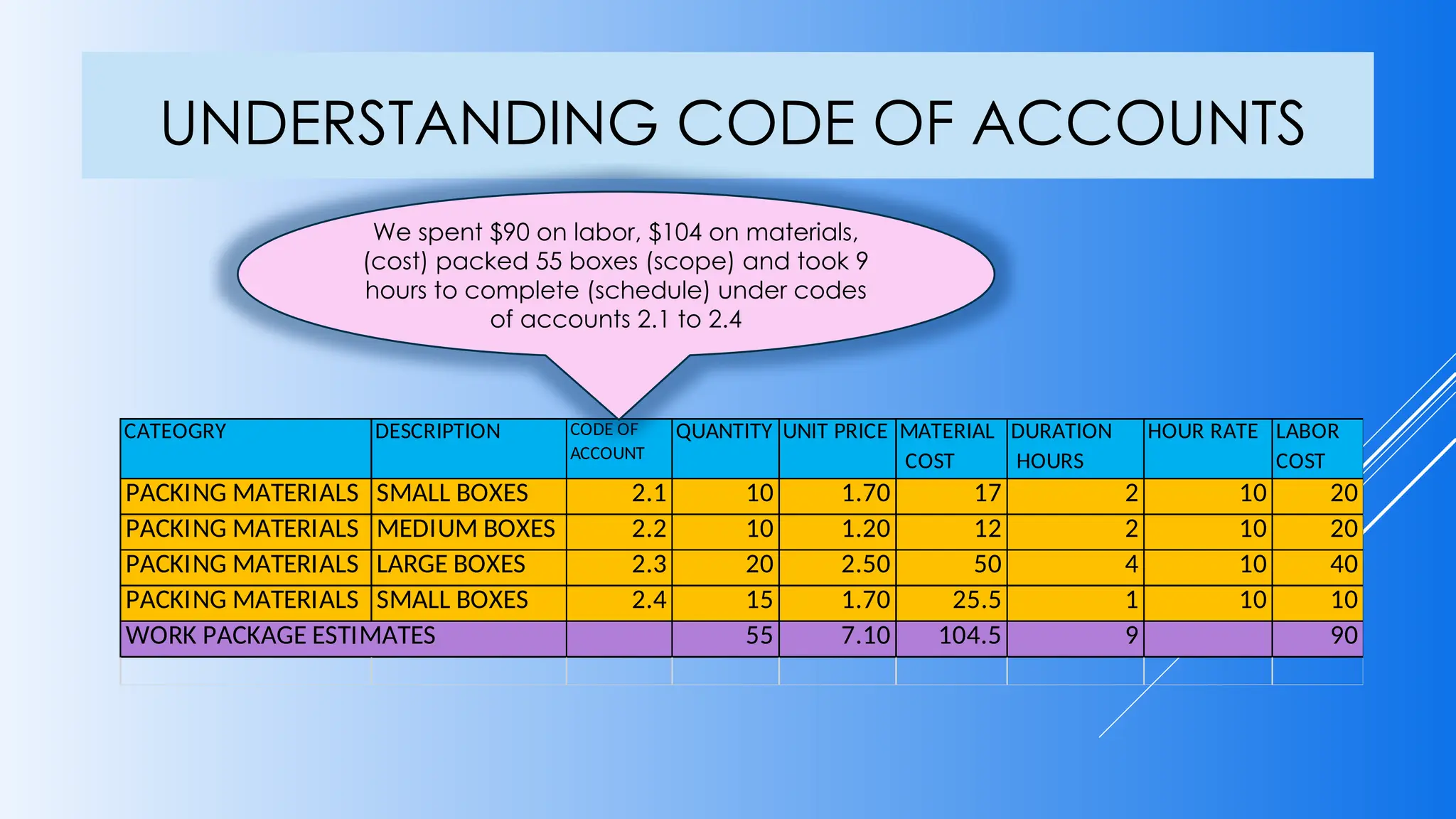
MARKS IN YOUR POCKET
A BRAIN DUMP FOR PMP STUDIES
Pic credit: Jenny goldstein
SCOPE MANAGEMENT
UNDERSTANDING CODE OF ACCOUNTS
CATEOGRY DESCRIPTION CODE OF
ACCOUNT
QUANTITY UNIT PRICE $
MATERIAL
COST
DURATION
HOURS
HOUR RATE LABOR
COST
PACKING MATERIALS SMALL BOXES 2.1 10 1.70 17 2 10 20
PACKING MATERIALS MEDIUM BOXES 2.2 10 1.20 12 2 10 20
PACKING MATERIALS LARGE BOXES 2.3 20 2.50 50 4 10 40
PACKING MATERIALS SMALL BOXES 2.4 15 1.70 25.5 1 10 10
WORK PACKAGE ESTIMATES 55 7.10 104.5 9 90
We spent $90 on labor, $104 on materials,
(cost) packed 55 boxes (scope) and took 9
hours to complete (schedule) under codes
of accounts 2.1 to 2.4
PDM RELATIONSHIPS
INSTAL OS
PERFORM TESTS
CONDUT LESSONS
LEARNED MEETING
COMPLETE
PROJECT FILE
BEGIN DAY SHIFT
END NIGHT SHIFT
FINISH TO START
START TO START FINISH TO FINISH
START TO FINISH
CONFIGURE HARDWARE
DOCUMENT TEST
RESULTS
DEPENDENCY DETERMINATION
MANDATORY DEPENDENCY
Relationship between activities that is legal, contractual
Some times due to physical limitations inherent in the nature of work
Also called hard logic
Example : Activity 1: Scrap old paint;
Activity 2: Apply new paint.
DISCRETIONARY DEPENDENCY
Based on subject matter expertise in application area and past experience
Also called soft logic or preferred logic
Discretionary dependencies should be fully documented so that fast tracking options
can be explored later in project. Documenting a discretionary dependency as
mandatory dependency, erroneously, can result in arbitrary float values in schedule.
Example: Activity 1: Paint Interior Wall;
Activity 2: Paint Exterior Wall.
DEPENDENCY DETERMINATION
EXTERNAL DEPENDENCY
Involves relationship between project activities and non project activities.
Could be beyond the control of project team
EXAMPLE:
Activity 1: Get townhall approval;
Activity 2: Lay foundation
INTERNAL DEPENDENCY
Fully within control of project team
Example:
Activity A : Write Code;
Activity B: Perform Unit Test
LEADS & LAGS
 Lead means advancing a successor
activity by a certain amount of
time.
 Lead could result in shortening of
schedule
 Example: Activity A: Prepare
Ground; Activity B: Landscape
 F –S 3 DAYS LEAD
PREPARE GROUND
LANDSCAPE
LEAD: 3 DAYS
5 DAYS
5 DAYS
 Lag means delaying successor activity.
 Lag could extend schedule duration
 S-S 3 DAYS LAG
5 DAYS
PREPARE GROUND
LANDSCAPE
LAG : 3 DAYS
5 DAYS
TOTAL : 5 +3 = 8 DAYS
LEADS & LAGS
 THREE POINT ESTIMATING
 Single point estimates do not
consider uncertainty conditions.
 Three point estimates combines
optimistic, most likely and
pessimistic scenarios
 There are two types of three point
estimates
THREE POINT ESTIMATING
 ANALOGOUS ESTIMATING
 Uses historical data of past similar
projects, such as budget, duration,
size etc.
 Adjusts the data based on the
known differences of current
project complexity
 Applied when there is limited
amount of information
 Also called as gross value
estimating approach
 Should be used by people with
expertise in application knowledge
area
 PARAMETRIC ESTIMATING
 Uses algorithm based on past
projects to estimation durations.
 Example: No. of labour hours for
constructing 1 metre of wall.
 Uses statistical relationships in past
projects
THREE POINT ESTIMATING
WHEN TO USE
 RESERVE ANALYSIS – Used to determine
amount of contingent and
management reserves required in
duration estimates.
 CONTINGENCY RESERVES: For identified,
accepted, known risks which is part of
cost baseline. (Known Unknown)
 This duration is estimated for unknown
amount of rework
 Contingency reserve can be removed
from individual activity and
aggregated.
 Contingency reserve should be clearly
identified in schedule documentation
 MANAGEMENT RESERVE:
 An amount of project budget or project
schedule held outside of the performance
measurement baseline (PMB) for management
control purpose, that is reserved for unforeseen
work that is within scope of the project.
 This is also for unknown risks (unknown
unknowns)
 As these are for activities which cannot be
scheduled, management reserve is not
therefore part of schedule baseline, but is within
the overall project duration or project budget.
 Use of management reserve may require a
change to the baseline.
RESERVE ANALYSIS
 Fist of Five voting - The project
manager asks the team to show
their level of support. This is a
method of getting quick vote.
 1 finger : No Way. Block proposal.
 2 fingers: I have some concerns. We
must resolve it before I support it.
 3 fingers: I will support this idea. But
some concerns. Still will move on.
 4 fingers: I support this idea, sounds
Good
 5 fingers: Absolutely best idea
ever ! I will champion it.
DECISION MAKING - VOTING
S
5 6 2
2 2
F
A B C
D E
5
F
1 5 6 11 12 13
1 2 3 4
14 18
14 18
12 13
6 11
1 5
10 11 12 13
FREE FLOAT = ff =
Earliest start of all successor activities (-) ES of activity(-)
Duration of activity
TF = 0
FF = 6-1-5=0
TF = 0
FF =12-6-6=0
TF = 0
FF = 14-12-2=0
TF = 0
FF – 19 (?)-14-5=0
TF = 9
FF =3-1-2=0
TF = 9
FF =14-3-2=9
Free float is the amount of time you can delay any activity without delaying the
earliest start of any succeeding activity. Notice that it doesn’t mention anything about
the final end date of the project or duration.
TOTAL FLOAT = tf = LF-EF or LS-ES
Total float is the amount of time an activity can be delayed from its
early start date without delaying the project finish date.
DEVELOP SCHEDULE – TOTAL & FREE FLOATS
S
5 6 2
2 2
F
A B C
D E
5
F
1 5 6 11 12 13
1 2 3 4
14 18
14 18
12 13
6 11
1 5
10 11 12 13
Schedule constraint
Causes : Resource levelling,
must finish dates, multiple
project calendars etc
0
0
0
0
9
9
POSITIVE TOTAL FLOAT or NEGATIVE TOTAL FLOAT is the difference between schedule
constraint and early finish for project.
DEVELOP SCHEDULE –POSITIVE & NEGATIVE
TOTAL FLOATS
RESOURCE OPTIMIZATION
 RESOURCE LEVELLING
 Technique applied when Resource is over allocated for more than one activity during the same
period or when there is a need to keep resource usage at constant level.
 Resource levelling can often cause critical path to change
 Available float is used for levelling resources.
W
T F S S M
8 8
8
8
W
T F S S M
8 8
8
8
BOB
BOB
BOB
Before levelling After levelling
M
T W T
6 7 5 6
M
T W T
6 6 6 6
No predetermined limits fixed Predetermined limit 6 hours fixed within available float
• RESOURCE SMOOTHING
• Method to ensure requirement for resource does not exceed certain pre-determined
resource limits.
• It is done only within their total float.
• Since it is done within available float, schedule will not get delayed and critical path will not
change.
RESOURCE OPTIMIZATION
BEFORE SMOOTHING AFTER SMOOTHING
SCHEDULE COMPRESSION
FAST TRACKING : Performing activities in parallel.
Increases risk of rework and quality.
Involves greater coordination among activities being fast tracked.
1 2 3 4 5
6 7 8 9 10
1 2 3 4 5
3 4 5 6 7
NORMAL
FAST
TRACKING
HIGH RISK
SCHEDULE COMPRESSION
 CRASHING: Shorten schedule duration by adding resources, Through approving overtime and adding
resources.
 Crashing works only on critical paths. Crashing may increase cost.
 Crashing works only for activities that effort driven. Compare crashing with fast tracking
1 2 3 4 5
3 4 5 6 7
FAST
TRACKING
HIGH RISK
1 2 3
4 5
CRASHING
HIGH COST
The project schedule shows a duration of 47 weeks
Customer has advanced the constraint by 5 weeks.
You are asked to consider crashing the schedule appropriately
There are 5 activities on the critical path that can be crashed
Current duration Weeks saved by crashing Cost of crashing
A 8 2 4000
F 9 4 16000
J 12 1 2000
K 5 2 2000
R 8 3 9000
ANSWERS : Crashing required only for 5 weeks
Option A A+J+K 4000+2000+2000 8000
Option B F+J 16000 + 2000 18000
Option C A+R 4000+9000 13000
Option D K+R 2000+9000 11000
ANSWER: OPTION A IS THE LEAST EXPENSIVE
PROBLEM IN CRASHING
RELEASE PLAN (FEATURES)
RELEASE 1
FEATURES
Iteration
0
Iteration
1
Iteration
2
Iteration
3
Iteration
n
ITERATION PLAN
FEATURE A FEATURE B FEATURE C FEATURE D
USER STORY 1 (20
STORY POINTS )
USER STORY 2 ( 5
STORY POINTS)
PRODUCT VISION DRIVES PRODUCT ROADMAP
PRODUCT ROADMAP DRIVES RELEASE PLANS
RELEASE PLAN ESTABLISHES ITERATIONS
ITERATION PLANS SCHEDULE FEATURE
DEVELOPMENT
PRIORITIZED FEATURES DELIVERED BY USER
STORIES (ESTIMATED IN STORY POINTS)
TASKS (ESTIMATED IN HOURS) CREATED TO
DELIVER USER STORIES
PRODUCT ROAD MAP EPICS
RELEASE 2
FEATURES
RELEASE 3
FEATURES
VISION
A
G
I
L
E
R
E
L
E
A
S
E
P
L
A
N
N
I
N
G
TASK: BUSINESS RULES 18 HOURS
TASK : U.I.PROTOTYPE 4 HOURS
TASK : ACTIVITY DIAGRAM 2 HOURS
TASK : REFACTORING 4 HOURS
TASK: DATA BASE PROC 3 HOURS
PLAN QUALITY MANAGEMENT
• Benchmarking
• Involves comparing planned projects with comparable projects to identify best
practices and set standards for improvement.
• Cost of quality
• Cost of conformance
• Prevention costs – documenting quality processes, giving right time, tools and
investing in training team resources.
• Appraisal costs – Testing
• Cost of non conformance
• Internal failure costs – rework, scrap
• External failure costs – liability, lost business, warranty costs.
• Flow Charts
• Helps anticipate where quality problems could occur and incorporate quality checks.
• SPIOC model helps establish value chain.
• Helps establish monetary value of cost of quality.
PLAN QUALITY MANAGEMENT
• Quality & Grade
• Quality – conformance to requirements
• Grade – deliverables distinguished based on different technical specifications but
having same functional use.
• Prevention over inspection
• Prevention is keeping errors out of the process, inspection is keeping errors out of the
customers hands
• Attribute Sampling & Variable sampling
• Attribute sampling – Results either conform or does not confirm
• Variable sampling – Results are rated on a continuous scale to measure degree of
conformity
• Tolerances and Control limits –
• Tolerances – specified range of acceptable limits
• Control limits – boundaries of common variation in a statistically stable process
PLAN QUALITY MANAGEMENT
• Logical data model
• Logical data model visually lays down organization’s data.
• This is independent of any technology
• Used to identify data integrity issues
• Matrix diagram
• Helps in identifying quality metrics for any quality management system
• Different quality attributes could be caused by different factors.
• The attributes and factors are laid down as rows and columns to indicate strength of
relationship.
• Mind mapping
• Useful for rapid gathering information about quality requirements, constraints,
dependencies and relationships.
MANAGE QUALITY
• Affinity diagram – shows potential causes of defects into groups showing areas that should
be focussed most.
• Histogram – represents numerical defects data in histograms.
• Scatter diagram – shows relationship between process on one hand and quality defect on
the other hand.
• DfX – technical guidelines that will help optimize specific aspects of design.
CONTROL QUALITY
• Check list – used to verify that quality processes have been performed or quality attributes
are present in deliverables.
• Check sheet – also called Tally sheet – Structured template used to collect defect data.
• Statistical sampling – choosing a part of the population of deliverables for inspection.
• Questionnaires & Surveys –Used to gather customer feedback after deployment or delivery
of a product.
• Control Charts – Used to verify stability and consistency of a process.
• Out of order – Process is out of order if 7 consecutive values occur on one side of the
mean (or) if any value touches control limit.
• When process is out of order, special cause should be investigated.
• When values occur on both sides of the mean in random or chance, this is normal and
can be ignored.
RESOURCE MANAGEMENT
Resource management methods
• Lean Management – based on 3 principles
• Eliminate waste
• Deliver value from customer’s perspective
• Continuous improvement
• Just-in-time Manufacturing
• Production is done just for demand in hand and not in anticipation of need.
• 3 of the 7 forms of waste, viz;, over production, waiting time and excess inventory is
avoided.
• Total Productive Maintenance
• Operators of machines maintain their own equipment.
• Traditional barriers between operations teams and maintenance crew is removed.
• Benefits: No breakdowns, no small stops, No defects, No accidents.
RESOURCE MANAGEMENT
Resource management methods
• Theory of constraints
• In any production process there will be constraints
• TOC focusses on removing these constraints by focussing on the rest of the processes
• The rest of the processes are subordinated to remove the constraints
• If it still does not work, only then add capacity, no automatically.
• Repeat the process until all constraints are released.
• Constraints could be lack of machine capacity, lack of training, etc, that limits system
capacity.
RESOURCE MANAGEMENT
Tuckman’s Ladder
• Forming – Team members meet and learn about their roles – Team members tend to be
independent and not open
• Storming – Team members start work on projects, discuss management and technical
approaches. Team members must collaborate and be open to different perspectives, else
will become counterproductive.
• Norming – team members start to worth together and support each other.
• Performing – Teams are well organized, inter dependent and work through issues smoothly
and effectively.
• Adjourning – Team comples the work and moves on.
MARKS IN YOUR POCKET
A BRAIN DUMP FOR PMP STUDIES
Pic credit: Jenny goldstein
COST MANAGEMENT
TRIANGULAR DISTRIBUTION
(P + ML + O)/3
EXAMPLE
You are driving to the airport to catch the 10 am flight to New York. You will be leaving
to airport by 7 am. You are confident of reaching airport in 60 minutes. If the traffic is
light you may reach there in 30 minutes. If there are too many vehicles on the road it is
likely to take even 120 minutes. What is the expected time of your arrival at airport
based on three point estimate (triangular distribution)
ANSWER
(120 + 60+ 30) /3 = 210/3 = 70
EXPECTED TIME OF ARRIVAL : 8.10 AM
SCHEDULE MANAGEMENT
EXAMPLE
You are driving to the airport to catch the 10 am flight to New York. You will be leaving
to airport by 7 am. You are confident of reaching airport in 60 minutes. If the traffic is
light you may reach there in 30 minutes. If there are too many vehicles on the road it is
likely to take even 120 minutes. What is the expected time of your arrival at airport
based on three point estimate (triangular distribution)
ANSWER
(120 +(4*60)+ 30) /6 = 390/6 = 65
EXPECTED TIME OF ARRIVAL : 8.05 AM
PERT OR BETA DISTRIBUTION
(P + (4*ML) + O)/6
SCHEDULE MANAGEMENT
STANDARD DEVIATION
INDICATES THE RANGE OF VALUES THAT DEVIATE FROM THE MEAN
(P-O)/6
EXAMPLE
From the following values ascertain standard deviation
Pessimistic 120; Optimistic 60; Most likely 30
The PERT is 70
ANSWER
(120-30)/6 = 90/6 = 15
Standard Deviation = 70 +/- 15
SCHEDULE MANAGEMENT
S
5 6 2
2 2
F
A B C
D E
5
F
1 5 6 11 12 13
1 2 3 4
14 18
14 18
12 13
6 11
1 5
10 11 12 13
TF = 0
FF = 6-1-5=0
TF = 0
FF =12-6-6=0
TF = 0
FF = 14-12-2=0
TF = 0
FF – 19 (?)-14-5=0
TF = 9
FF =3-1-2=0
TF = 9
FF =14-3-2=9
FREE FLOAT = ff =
Earliest start of all successor activities (-) ES of activity
(-) Duration of activity
NOTICE DIFFERENCE: Free float is the amount of time you can delay any activity without delaying the earliest start of any
succeeding activity. It doesn’t mention anything about the final end date of the project or duration.
TOTAL FLOAT = tf = LF-EF or LS-ES
Total float is the amount of time an activity can be delayed from its
early start date without delaying the project finish date.
SCHEDULE MANAGEMENT
RANGE – BASIS OF ESTIMATES
A range of 2 weeks +/- 2 days assuming a 5 day work week gives a range of __
ANSWER
At least 8 days and not more than 12 days
EXAMPLE
SCHEDULE MANAGEMENT
1 2 3 4
5
4
3
2
1
0
ES
AT
AC
PV
PD
SV = EV-PV
CV =EV-AC
SPI(t) = ES/AT
EV
EAC (t) = PD/SPI
BAC
$
COST MANAGEMENT
You must be able to
interpret these lines :
• Planned value
• Earned Value
• Actual Cost
• BAC
• Earned Schedule
• Actual Time
• Planned Duration
 FORMULAS
 CV = EV – AC
 CPI = EV/AC
 SV = EV – PV
 SPI = EV/PV
 EAC = BAC/CPI (If CPI is expected to be same for
remainder project)
 EAC = AC (BAC-EV) (If future work is expected to be
accomplished at planned rate)
 EAC = AC + (BOTTOM UP RE-ESTIMATE) (If actual plan is
no longer valid)
 EAC = AC +(BAC-EV)/ (CPI * SPI) (When both CPI and SPI
is expected to influence future performance)
 VAC = BAC – EAC
 TCPI = (BAC-EV)/(EAC-AC)
 TCPI = (BAC-EV)/BAC-AC)
• ABBREVIATIONS USED
• PV= Authorized budget for a given quantum of
work.
• EV= Work performed measured against
planned value (budget authorized) for that
quantum of work.
• AC = Amount expended
• CV= Cost Variance
• CPI= Cost performance index
• SV = Schedule variance
• SPI = Schedule Performance index
• EAC = Estimate at Completion
• AC = Actual Cost
• VAC = Variance at completion
• TCPI = To Complete Performance Index
COST MANAGEMENT-EVM
• ABBREVIATIONS USED
• SAC – Schedule at Completion. This is the original planned completion date of the
project.
• SAC is also referred as PD or Planned duration.
• ES – Duration from the beginning of the project till current date when earned
value’s equivalent date in planned value will be established.
• AT – This is the duration from beginning of the project to status date.
• PAR – Planned Accomplishment Rate which is the average planned value period
schedule period.
• PAR = BAC / SAC or BAC / PD
• SV can be transformed to time units by dividing SV by PAR
• SV(T) = SV/PAR
• SPI(T) = ES/AT
COST MANAGEMENT - ES
EARNED VALUE MANAGEMENT
 CV
 POSITIVE – UNDER BUDGET
 NEGATIVE – OVER BUDGET
 ZERO – ON TARGET
 CPI
 >1 – UNDER BUDGET
 =1 – AS PLANNED
 <1 – OVER BUDGET
EARNED SCHEDULE
 SV
 >1 AHEAD OF SCHEDULE
 =1 ON SCHEDULE
 <1 BEHIND SCHEDULE
 SPI
 >1 AHEAD OF SCHEDULE
 =1 ON SCHEDULE
 <1 BEHIND SCHEDULE
COST MANAGEMENT
 FORMULAS
 SV (t) = ES – AT
 SPI (t) = ES/AT
 IEAC (t) = PD/SPI (t) (when current SPI
(t) is expected to continue.
 IEAC (t) AT + (PD-ES)/SPI(t) (when
initially planned rate of performance
will apply for future period)
 VAC (t) = PD – EAC (t)
 ETC = EAC (t) - PD
• ABBREVIATIONS USED
• ES = Earned Schedule. Amount of
schedule work earned on a reference
date.
• AT = Actual time. Duration from
beginning of project till status date.
• PAR = BAC/ PD. Gives average PV per
time period, called Planned
Accomplishment Rate.
• PD – Planned Duration
• IEAC (t) Independent Estimate at
Completion (ttime).
• VAC (t) = Variance at completion
Time estimate is based on time, not cost.
COST MANAGEMENT
RANGE – BASIS OF ESTIMATES
A range of 2 weeks +/- 2 days assuming a 5 day work week gives a range of __
ANSWER
At least 8 days and not more than 12 days
EXAMPLE
COST MANAGEMENT
COST MANAGEMENT
Rough Order of Magnitude estimate (ROM) = -25% / + 75%
(Initiation stage of project)
Definitive range of estimates -5% / + 10%
(when activity level details are understood)
CHANNELS OF COMMUNICATIONS
C = N (N-1)/2
COMMUNICATIONS MANAGEMENT
EMV = PROBABILITY * IMPACT
RISK MANAGEMENT
FIXED PRICE
COST
REIMBURSABL
E
TIME &
MATERIAL
PURCHASE
ORDER
contracts
CONTRACTS – COST REIMBURSABLE
• COST REIMBURSABLE CONTRACTS
• All seller’s cost are reimbursed by the buyer, Seller’s profit stated as Fee is
included.
• Cost is unknown at the beginning
• Buyer has the most cost risk, so generally bad for any buyer
• Used when precise description of goods or services cannot be developed
• Seller is responsible for detailing the scope of work
CONTRACTS – COST REIMBURSABLE
• CPFF: Actual Cost = $ 100,000 Fee = $ 10,000 Total buyer pays to Seller = 110,000
• CPPC: Actual Cost = $ 100,000 Fee = 25% of the cost Total buyer pays to Seller = 100,000 + 25% of 100,000 = 125,000
• Cost Plus Incentive Fee (CPIF)
• Target Cost: $100,000
• Fee: $10,000
• Share Ratio: 80/20 (Buyer/Seller)
• Actual Cost + Fee + ((Target Cost - Actual Cost) * Share Ratio)
• Scenario 1: Actual Cost: $80,000
• Seller receives: $80,000 + $10,000 + (20,000 * 20%) = $ 94,000
• Scenario 2: If Actual Cost: $120,000
• Seller receives: $120,000 + $10,000 + (-20,000 * 20%) = $126,000
• CPAF – Cost Plus Award Fee
Similar with CPIF, but the bonus is based on meeting specified performance metrics
Based on sole discretion of buyer, generally not subject to appeals.
INCENTIVE WITH CEILING
(Fixed Price, Incentive fee
with ceiling)
Target cost $ 5.00 M
Target fee $ 1.00 M
Target price $ 5.00 + $ 1.00 = $ 6.00 M
Ceiling price $ 8.00 M
Buyers/Sellers share ratio 80:20
Point of Total Assumption =
Target cost + ( (Ceiling price - Target Price)*Buyers
Share
5.00 + ((8.00 – 6.00)*80%)
=5.00 + (2.00*80%)
= 5.00 +1.60
= 6.60
Point of Total Assumption is $ 6.60 M
Buyer need not pay beyond this limit. Seller
assumes 100 % responsibility from this point.
Target cost 5.00
Target fee 1.00
Target price 6.00
CEILING 8.00
O
V
E
R
R
U
N
PTA = 5 + (8.00 – 6.00) / 0.80
= 6.60
SELLER TAKES EVERY $
FROM THIS POINT
49
CONTRACTS – FIXED PRICE
• FIXED PRICE CONTRACT
• The most common form of contract
• Appropriate when buyer can describe the scope of work
• Has the least cost risk for the buyer
• Types of FP contracts:
• FFP – Firm Fixed price
• FPIF – Fixed Price Incentive Fee with ceiling ( we will discuss Point of Total
Assumption)
• FP-EPA – Fixed Price Economic Price Adjustment
CONTRACTS – FIXED PRICE
• FIXED PRICE
• FFP – Firm Fixed price
• The most common form of contract
• Appropriate when buyer can describe the scope of work
• Has the least cost risk for the buyer
• FPIF – Fixed Price Incentive Fee ( FIXED BECAUSE OF CEILING PRICE – see PTA slide)
• Allow flexibility. Permits deviation from a target price.
• Incentives for performing within targeted price, schedule or technical performance metrics.
• FP-EPA – Fixed Price Economic Price Adjustment
• When contracts are for long term
• Or When foreign currency is involved
• When allowance needs to be provided for inflation or cost increase beyond supplier’s control
• Allow for changes to final price based on economic indicators.
51
CONTRACTS - HYBRID
 TIME & MATERIAL CONTRACT
 Sometimes called Unit Price
 The price is per hour or per item
 Usually used for small amounts
 A combination of Fixed Price and Cost Reimbursable
 Fixed price per item
 The total cost is unknown, varying with the amount of materials or time
CONTRACTS
T&M CPFF CPAF CPIF FPIF FPEPA FFP
Buyer Low
High
Seller
Low High
Risk by Type of Contract – Buyer Vs Seller
PROJECT PROCUREMENT
MANAGEMENT - AGILE
• In traditional projects, scope can
be determined early and SOW can
also be drawn up at that time for
the procurement work packages.
• In agile projects, scope is
determined only at the beginning
of iteration and light weight SOWs
are drawn.
• Fitness for business purpose and
not original specifications, will
drive acceptance criteria.
PARADIGM SHIFT
PROJECT PROCURMENT
MANAGEMENT
CONSIDERATIONS FOR AGILE
Specific sellers may be used to
form an agile team.
Shared risk-reward models are
used.
In larger projects, a stable
approach may be used for some
deliverables and an adaptive
approach for others.
A Master Services Agreement
(MSA) for the overall work with
appendices for adaptive work
could be used.
Changes to adaptive work can
progress without impacting
overall contract.
CONTRACT
Master
service
agreement
Part a:
features
(subject to
review &
change)
Part b:
Parties
involved,
terms &
conditions
PART A:
Schedule of
services
PART B:
Schedule of
services
Statement of
work
Statement of
work
Statement of
work
55
Contract Type Description
Capped Time and
Materials Contracts
• Works like traditional Time and Materials contracts.
• However, an upper limit is set on customers’ payment.
• Customers pay up for the capped cost limit.
• Suppliers benefit in case of early time-frame changes.
(*)
Incremental Delivery
Contracts
• Customers review contracts during the contract life
cycle at pre-negotiated designated points of the
contract lifecycle.
• Customers can make required changes, continue or
terminate the project at these points.
Other Agile Contract Types
*Money for nothing, change for free
INCENTIVE WITH CEILING
(FIXED PRICE, INCENTIVE
FEE WITH CEILING)
• Target cost $ 5.00 M
• Target fee $ 1.00 M
• Target price $ 5.00 + $ 1.00 = $ 6.00 M
• Ceiling price $ 8.00 M
• Buyers/Sellers share ratio 80:20
• Point of Total Assumption =
• Target cost + ( (Ceiling price - Target
Price)*Buyers Share
• 5.00 + ((8.00 – 6.00)*80%)
• =5.00 + (2.00*80%)
• = 5.00 +1.60
• = 6.60
• Point of Total Assumption is $ 6.60 M
• Buyer need not pay beyond this limit. Seller
assumes 100 % responsibility from this point.
Target cost 5.00
Target fee 1.00
Target price 6.00
O
V
E
R
R
U
N
SELLER TAKES EVERY $
FROM THIS POINT
CEILING 8.00
PTA = 5 + (8.00 – 6.00) / 0.80
= 6.60

MARKS IN YOUR POCKET PMP for PMP Preparation

  • 1.
    MARKS IN YOURPOCKET A BRAIN DUMP FOR PMP STUDIES Pic credit: Jenny goldstein
  • 2.
  • 3.
    UNDERSTANDING CODE OFACCOUNTS CATEOGRY DESCRIPTION CODE OF ACCOUNT QUANTITY UNIT PRICE $ MATERIAL COST DURATION HOURS HOUR RATE LABOR COST PACKING MATERIALS SMALL BOXES 2.1 10 1.70 17 2 10 20 PACKING MATERIALS MEDIUM BOXES 2.2 10 1.20 12 2 10 20 PACKING MATERIALS LARGE BOXES 2.3 20 2.50 50 4 10 40 PACKING MATERIALS SMALL BOXES 2.4 15 1.70 25.5 1 10 10 WORK PACKAGE ESTIMATES 55 7.10 104.5 9 90 We spent $90 on labor, $104 on materials, (cost) packed 55 boxes (scope) and took 9 hours to complete (schedule) under codes of accounts 2.1 to 2.4
  • 4.
    PDM RELATIONSHIPS INSTAL OS PERFORMTESTS CONDUT LESSONS LEARNED MEETING COMPLETE PROJECT FILE BEGIN DAY SHIFT END NIGHT SHIFT FINISH TO START START TO START FINISH TO FINISH START TO FINISH CONFIGURE HARDWARE DOCUMENT TEST RESULTS
  • 5.
    DEPENDENCY DETERMINATION DEPENDENCY DETERMINATION MANDATORYDEPENDENCY Relationship between activities that is legal, contractual Some times due to physical limitations inherent in the nature of work Also called hard logic Example : Activity 1: Scrap old paint; Activity 2: Apply new paint. DISCRETIONARY DEPENDENCY Based on subject matter expertise in application area and past experience Also called soft logic or preferred logic Discretionary dependencies should be fully documented so that fast tracking options can be explored later in project. Documenting a discretionary dependency as mandatory dependency, erroneously, can result in arbitrary float values in schedule. Example: Activity 1: Paint Interior Wall; Activity 2: Paint Exterior Wall.
  • 6.
    DEPENDENCY DETERMINATION DEPENDENCY DETERMINATION EXTERNALDEPENDENCY Involves relationship between project activities and non project activities. Could be beyond the control of project team EXAMPLE: Activity 1: Get townhall approval; Activity 2: Lay foundation INTERNAL DEPENDENCY Fully within control of project team Example: Activity A : Write Code; Activity B: Perform Unit Test
  • 7.
    LEADS & LAGS Lead means advancing a successor activity by a certain amount of time.  Lead could result in shortening of schedule  Example: Activity A: Prepare Ground; Activity B: Landscape  F –S 3 DAYS LEAD PREPARE GROUND LANDSCAPE LEAD: 3 DAYS 5 DAYS 5 DAYS
  • 8.
     Lag meansdelaying successor activity.  Lag could extend schedule duration  S-S 3 DAYS LAG 5 DAYS PREPARE GROUND LANDSCAPE LAG : 3 DAYS 5 DAYS TOTAL : 5 +3 = 8 DAYS LEADS & LAGS
  • 9.
     THREE POINTESTIMATING  Single point estimates do not consider uncertainty conditions.  Three point estimates combines optimistic, most likely and pessimistic scenarios  There are two types of three point estimates THREE POINT ESTIMATING
  • 10.
     ANALOGOUS ESTIMATING Uses historical data of past similar projects, such as budget, duration, size etc.  Adjusts the data based on the known differences of current project complexity  Applied when there is limited amount of information  Also called as gross value estimating approach  Should be used by people with expertise in application knowledge area  PARAMETRIC ESTIMATING  Uses algorithm based on past projects to estimation durations.  Example: No. of labour hours for constructing 1 metre of wall.  Uses statistical relationships in past projects THREE POINT ESTIMATING
  • 11.
  • 12.
     RESERVE ANALYSIS– Used to determine amount of contingent and management reserves required in duration estimates.  CONTINGENCY RESERVES: For identified, accepted, known risks which is part of cost baseline. (Known Unknown)  This duration is estimated for unknown amount of rework  Contingency reserve can be removed from individual activity and aggregated.  Contingency reserve should be clearly identified in schedule documentation  MANAGEMENT RESERVE:  An amount of project budget or project schedule held outside of the performance measurement baseline (PMB) for management control purpose, that is reserved for unforeseen work that is within scope of the project.  This is also for unknown risks (unknown unknowns)  As these are for activities which cannot be scheduled, management reserve is not therefore part of schedule baseline, but is within the overall project duration or project budget.  Use of management reserve may require a change to the baseline. RESERVE ANALYSIS
  • 13.
     Fist ofFive voting - The project manager asks the team to show their level of support. This is a method of getting quick vote.  1 finger : No Way. Block proposal.  2 fingers: I have some concerns. We must resolve it before I support it.  3 fingers: I will support this idea. But some concerns. Still will move on.  4 fingers: I support this idea, sounds Good  5 fingers: Absolutely best idea ever ! I will champion it. DECISION MAKING - VOTING
  • 14.
    S 5 6 2 22 F A B C D E 5 F 1 5 6 11 12 13 1 2 3 4 14 18 14 18 12 13 6 11 1 5 10 11 12 13 FREE FLOAT = ff = Earliest start of all successor activities (-) ES of activity(-) Duration of activity TF = 0 FF = 6-1-5=0 TF = 0 FF =12-6-6=0 TF = 0 FF = 14-12-2=0 TF = 0 FF – 19 (?)-14-5=0 TF = 9 FF =3-1-2=0 TF = 9 FF =14-3-2=9 Free float is the amount of time you can delay any activity without delaying the earliest start of any succeeding activity. Notice that it doesn’t mention anything about the final end date of the project or duration. TOTAL FLOAT = tf = LF-EF or LS-ES Total float is the amount of time an activity can be delayed from its early start date without delaying the project finish date. DEVELOP SCHEDULE – TOTAL & FREE FLOATS
  • 15.
    S 5 6 2 22 F A B C D E 5 F 1 5 6 11 12 13 1 2 3 4 14 18 14 18 12 13 6 11 1 5 10 11 12 13 Schedule constraint Causes : Resource levelling, must finish dates, multiple project calendars etc 0 0 0 0 9 9 POSITIVE TOTAL FLOAT or NEGATIVE TOTAL FLOAT is the difference between schedule constraint and early finish for project. DEVELOP SCHEDULE –POSITIVE & NEGATIVE TOTAL FLOATS
  • 16.
    RESOURCE OPTIMIZATION  RESOURCELEVELLING  Technique applied when Resource is over allocated for more than one activity during the same period or when there is a need to keep resource usage at constant level.  Resource levelling can often cause critical path to change  Available float is used for levelling resources. W T F S S M 8 8 8 8 W T F S S M 8 8 8 8 BOB BOB BOB Before levelling After levelling
  • 17.
    M T W T 67 5 6 M T W T 6 6 6 6 No predetermined limits fixed Predetermined limit 6 hours fixed within available float • RESOURCE SMOOTHING • Method to ensure requirement for resource does not exceed certain pre-determined resource limits. • It is done only within their total float. • Since it is done within available float, schedule will not get delayed and critical path will not change. RESOURCE OPTIMIZATION BEFORE SMOOTHING AFTER SMOOTHING
  • 18.
    SCHEDULE COMPRESSION FAST TRACKING: Performing activities in parallel. Increases risk of rework and quality. Involves greater coordination among activities being fast tracked. 1 2 3 4 5 6 7 8 9 10 1 2 3 4 5 3 4 5 6 7 NORMAL FAST TRACKING HIGH RISK
  • 19.
    SCHEDULE COMPRESSION  CRASHING:Shorten schedule duration by adding resources, Through approving overtime and adding resources.  Crashing works only on critical paths. Crashing may increase cost.  Crashing works only for activities that effort driven. Compare crashing with fast tracking 1 2 3 4 5 3 4 5 6 7 FAST TRACKING HIGH RISK 1 2 3 4 5 CRASHING HIGH COST
  • 20.
    The project scheduleshows a duration of 47 weeks Customer has advanced the constraint by 5 weeks. You are asked to consider crashing the schedule appropriately There are 5 activities on the critical path that can be crashed Current duration Weeks saved by crashing Cost of crashing A 8 2 4000 F 9 4 16000 J 12 1 2000 K 5 2 2000 R 8 3 9000 ANSWERS : Crashing required only for 5 weeks Option A A+J+K 4000+2000+2000 8000 Option B F+J 16000 + 2000 18000 Option C A+R 4000+9000 13000 Option D K+R 2000+9000 11000 ANSWER: OPTION A IS THE LEAST EXPENSIVE PROBLEM IN CRASHING
  • 21.
    RELEASE PLAN (FEATURES) RELEASE1 FEATURES Iteration 0 Iteration 1 Iteration 2 Iteration 3 Iteration n ITERATION PLAN FEATURE A FEATURE B FEATURE C FEATURE D USER STORY 1 (20 STORY POINTS ) USER STORY 2 ( 5 STORY POINTS) PRODUCT VISION DRIVES PRODUCT ROADMAP PRODUCT ROADMAP DRIVES RELEASE PLANS RELEASE PLAN ESTABLISHES ITERATIONS ITERATION PLANS SCHEDULE FEATURE DEVELOPMENT PRIORITIZED FEATURES DELIVERED BY USER STORIES (ESTIMATED IN STORY POINTS) TASKS (ESTIMATED IN HOURS) CREATED TO DELIVER USER STORIES PRODUCT ROAD MAP EPICS RELEASE 2 FEATURES RELEASE 3 FEATURES VISION A G I L E R E L E A S E P L A N N I N G TASK: BUSINESS RULES 18 HOURS TASK : U.I.PROTOTYPE 4 HOURS TASK : ACTIVITY DIAGRAM 2 HOURS TASK : REFACTORING 4 HOURS TASK: DATA BASE PROC 3 HOURS
  • 22.
    PLAN QUALITY MANAGEMENT •Benchmarking • Involves comparing planned projects with comparable projects to identify best practices and set standards for improvement. • Cost of quality • Cost of conformance • Prevention costs – documenting quality processes, giving right time, tools and investing in training team resources. • Appraisal costs – Testing • Cost of non conformance • Internal failure costs – rework, scrap • External failure costs – liability, lost business, warranty costs. • Flow Charts • Helps anticipate where quality problems could occur and incorporate quality checks. • SPIOC model helps establish value chain. • Helps establish monetary value of cost of quality.
  • 23.
    PLAN QUALITY MANAGEMENT •Quality & Grade • Quality – conformance to requirements • Grade – deliverables distinguished based on different technical specifications but having same functional use. • Prevention over inspection • Prevention is keeping errors out of the process, inspection is keeping errors out of the customers hands • Attribute Sampling & Variable sampling • Attribute sampling – Results either conform or does not confirm • Variable sampling – Results are rated on a continuous scale to measure degree of conformity • Tolerances and Control limits – • Tolerances – specified range of acceptable limits • Control limits – boundaries of common variation in a statistically stable process
  • 24.
    PLAN QUALITY MANAGEMENT •Logical data model • Logical data model visually lays down organization’s data. • This is independent of any technology • Used to identify data integrity issues • Matrix diagram • Helps in identifying quality metrics for any quality management system • Different quality attributes could be caused by different factors. • The attributes and factors are laid down as rows and columns to indicate strength of relationship. • Mind mapping • Useful for rapid gathering information about quality requirements, constraints, dependencies and relationships.
  • 25.
    MANAGE QUALITY • Affinitydiagram – shows potential causes of defects into groups showing areas that should be focussed most. • Histogram – represents numerical defects data in histograms. • Scatter diagram – shows relationship between process on one hand and quality defect on the other hand. • DfX – technical guidelines that will help optimize specific aspects of design.
  • 26.
    CONTROL QUALITY • Checklist – used to verify that quality processes have been performed or quality attributes are present in deliverables. • Check sheet – also called Tally sheet – Structured template used to collect defect data. • Statistical sampling – choosing a part of the population of deliverables for inspection. • Questionnaires & Surveys –Used to gather customer feedback after deployment or delivery of a product. • Control Charts – Used to verify stability and consistency of a process. • Out of order – Process is out of order if 7 consecutive values occur on one side of the mean (or) if any value touches control limit. • When process is out of order, special cause should be investigated. • When values occur on both sides of the mean in random or chance, this is normal and can be ignored.
  • 27.
    RESOURCE MANAGEMENT Resource managementmethods • Lean Management – based on 3 principles • Eliminate waste • Deliver value from customer’s perspective • Continuous improvement • Just-in-time Manufacturing • Production is done just for demand in hand and not in anticipation of need. • 3 of the 7 forms of waste, viz;, over production, waiting time and excess inventory is avoided. • Total Productive Maintenance • Operators of machines maintain their own equipment. • Traditional barriers between operations teams and maintenance crew is removed. • Benefits: No breakdowns, no small stops, No defects, No accidents.
  • 28.
    RESOURCE MANAGEMENT Resource managementmethods • Theory of constraints • In any production process there will be constraints • TOC focusses on removing these constraints by focussing on the rest of the processes • The rest of the processes are subordinated to remove the constraints • If it still does not work, only then add capacity, no automatically. • Repeat the process until all constraints are released. • Constraints could be lack of machine capacity, lack of training, etc, that limits system capacity.
  • 29.
    RESOURCE MANAGEMENT Tuckman’s Ladder •Forming – Team members meet and learn about their roles – Team members tend to be independent and not open • Storming – Team members start work on projects, discuss management and technical approaches. Team members must collaborate and be open to different perspectives, else will become counterproductive. • Norming – team members start to worth together and support each other. • Performing – Teams are well organized, inter dependent and work through issues smoothly and effectively. • Adjourning – Team comples the work and moves on.
  • 30.
    MARKS IN YOURPOCKET A BRAIN DUMP FOR PMP STUDIES Pic credit: Jenny goldstein COST MANAGEMENT
  • 31.
    TRIANGULAR DISTRIBUTION (P +ML + O)/3 EXAMPLE You are driving to the airport to catch the 10 am flight to New York. You will be leaving to airport by 7 am. You are confident of reaching airport in 60 minutes. If the traffic is light you may reach there in 30 minutes. If there are too many vehicles on the road it is likely to take even 120 minutes. What is the expected time of your arrival at airport based on three point estimate (triangular distribution) ANSWER (120 + 60+ 30) /3 = 210/3 = 70 EXPECTED TIME OF ARRIVAL : 8.10 AM SCHEDULE MANAGEMENT
  • 32.
    EXAMPLE You are drivingto the airport to catch the 10 am flight to New York. You will be leaving to airport by 7 am. You are confident of reaching airport in 60 minutes. If the traffic is light you may reach there in 30 minutes. If there are too many vehicles on the road it is likely to take even 120 minutes. What is the expected time of your arrival at airport based on three point estimate (triangular distribution) ANSWER (120 +(4*60)+ 30) /6 = 390/6 = 65 EXPECTED TIME OF ARRIVAL : 8.05 AM PERT OR BETA DISTRIBUTION (P + (4*ML) + O)/6 SCHEDULE MANAGEMENT
  • 33.
    STANDARD DEVIATION INDICATES THERANGE OF VALUES THAT DEVIATE FROM THE MEAN (P-O)/6 EXAMPLE From the following values ascertain standard deviation Pessimistic 120; Optimistic 60; Most likely 30 The PERT is 70 ANSWER (120-30)/6 = 90/6 = 15 Standard Deviation = 70 +/- 15 SCHEDULE MANAGEMENT
  • 34.
    S 5 6 2 22 F A B C D E 5 F 1 5 6 11 12 13 1 2 3 4 14 18 14 18 12 13 6 11 1 5 10 11 12 13 TF = 0 FF = 6-1-5=0 TF = 0 FF =12-6-6=0 TF = 0 FF = 14-12-2=0 TF = 0 FF – 19 (?)-14-5=0 TF = 9 FF =3-1-2=0 TF = 9 FF =14-3-2=9 FREE FLOAT = ff = Earliest start of all successor activities (-) ES of activity (-) Duration of activity NOTICE DIFFERENCE: Free float is the amount of time you can delay any activity without delaying the earliest start of any succeeding activity. It doesn’t mention anything about the final end date of the project or duration. TOTAL FLOAT = tf = LF-EF or LS-ES Total float is the amount of time an activity can be delayed from its early start date without delaying the project finish date. SCHEDULE MANAGEMENT
  • 35.
    RANGE – BASISOF ESTIMATES A range of 2 weeks +/- 2 days assuming a 5 day work week gives a range of __ ANSWER At least 8 days and not more than 12 days EXAMPLE SCHEDULE MANAGEMENT
  • 36.
    1 2 34 5 4 3 2 1 0 ES AT AC PV PD SV = EV-PV CV =EV-AC SPI(t) = ES/AT EV EAC (t) = PD/SPI BAC $ COST MANAGEMENT You must be able to interpret these lines : • Planned value • Earned Value • Actual Cost • BAC • Earned Schedule • Actual Time • Planned Duration
  • 37.
     FORMULAS  CV= EV – AC  CPI = EV/AC  SV = EV – PV  SPI = EV/PV  EAC = BAC/CPI (If CPI is expected to be same for remainder project)  EAC = AC (BAC-EV) (If future work is expected to be accomplished at planned rate)  EAC = AC + (BOTTOM UP RE-ESTIMATE) (If actual plan is no longer valid)  EAC = AC +(BAC-EV)/ (CPI * SPI) (When both CPI and SPI is expected to influence future performance)  VAC = BAC – EAC  TCPI = (BAC-EV)/(EAC-AC)  TCPI = (BAC-EV)/BAC-AC) • ABBREVIATIONS USED • PV= Authorized budget for a given quantum of work. • EV= Work performed measured against planned value (budget authorized) for that quantum of work. • AC = Amount expended • CV= Cost Variance • CPI= Cost performance index • SV = Schedule variance • SPI = Schedule Performance index • EAC = Estimate at Completion • AC = Actual Cost • VAC = Variance at completion • TCPI = To Complete Performance Index COST MANAGEMENT-EVM
  • 38.
    • ABBREVIATIONS USED •SAC – Schedule at Completion. This is the original planned completion date of the project. • SAC is also referred as PD or Planned duration. • ES – Duration from the beginning of the project till current date when earned value’s equivalent date in planned value will be established. • AT – This is the duration from beginning of the project to status date. • PAR – Planned Accomplishment Rate which is the average planned value period schedule period. • PAR = BAC / SAC or BAC / PD • SV can be transformed to time units by dividing SV by PAR • SV(T) = SV/PAR • SPI(T) = ES/AT COST MANAGEMENT - ES
  • 39.
    EARNED VALUE MANAGEMENT CV  POSITIVE – UNDER BUDGET  NEGATIVE – OVER BUDGET  ZERO – ON TARGET  CPI  >1 – UNDER BUDGET  =1 – AS PLANNED  <1 – OVER BUDGET EARNED SCHEDULE  SV  >1 AHEAD OF SCHEDULE  =1 ON SCHEDULE  <1 BEHIND SCHEDULE  SPI  >1 AHEAD OF SCHEDULE  =1 ON SCHEDULE  <1 BEHIND SCHEDULE COST MANAGEMENT
  • 40.
     FORMULAS  SV(t) = ES – AT  SPI (t) = ES/AT  IEAC (t) = PD/SPI (t) (when current SPI (t) is expected to continue.  IEAC (t) AT + (PD-ES)/SPI(t) (when initially planned rate of performance will apply for future period)  VAC (t) = PD – EAC (t)  ETC = EAC (t) - PD • ABBREVIATIONS USED • ES = Earned Schedule. Amount of schedule work earned on a reference date. • AT = Actual time. Duration from beginning of project till status date. • PAR = BAC/ PD. Gives average PV per time period, called Planned Accomplishment Rate. • PD – Planned Duration • IEAC (t) Independent Estimate at Completion (ttime). • VAC (t) = Variance at completion Time estimate is based on time, not cost. COST MANAGEMENT
  • 41.
    RANGE – BASISOF ESTIMATES A range of 2 weeks +/- 2 days assuming a 5 day work week gives a range of __ ANSWER At least 8 days and not more than 12 days EXAMPLE COST MANAGEMENT
  • 42.
    COST MANAGEMENT Rough Orderof Magnitude estimate (ROM) = -25% / + 75% (Initiation stage of project) Definitive range of estimates -5% / + 10% (when activity level details are understood)
  • 43.
    CHANNELS OF COMMUNICATIONS C= N (N-1)/2 COMMUNICATIONS MANAGEMENT
  • 44.
    EMV = PROBABILITY* IMPACT RISK MANAGEMENT
  • 45.
  • 46.
    CONTRACTS – COSTREIMBURSABLE • COST REIMBURSABLE CONTRACTS • All seller’s cost are reimbursed by the buyer, Seller’s profit stated as Fee is included. • Cost is unknown at the beginning • Buyer has the most cost risk, so generally bad for any buyer • Used when precise description of goods or services cannot be developed • Seller is responsible for detailing the scope of work
  • 47.
    CONTRACTS – COSTREIMBURSABLE • CPFF: Actual Cost = $ 100,000 Fee = $ 10,000 Total buyer pays to Seller = 110,000 • CPPC: Actual Cost = $ 100,000 Fee = 25% of the cost Total buyer pays to Seller = 100,000 + 25% of 100,000 = 125,000 • Cost Plus Incentive Fee (CPIF) • Target Cost: $100,000 • Fee: $10,000 • Share Ratio: 80/20 (Buyer/Seller) • Actual Cost + Fee + ((Target Cost - Actual Cost) * Share Ratio) • Scenario 1: Actual Cost: $80,000 • Seller receives: $80,000 + $10,000 + (20,000 * 20%) = $ 94,000 • Scenario 2: If Actual Cost: $120,000 • Seller receives: $120,000 + $10,000 + (-20,000 * 20%) = $126,000 • CPAF – Cost Plus Award Fee Similar with CPIF, but the bonus is based on meeting specified performance metrics Based on sole discretion of buyer, generally not subject to appeals.
  • 48.
    INCENTIVE WITH CEILING (FixedPrice, Incentive fee with ceiling) Target cost $ 5.00 M Target fee $ 1.00 M Target price $ 5.00 + $ 1.00 = $ 6.00 M Ceiling price $ 8.00 M Buyers/Sellers share ratio 80:20 Point of Total Assumption = Target cost + ( (Ceiling price - Target Price)*Buyers Share 5.00 + ((8.00 – 6.00)*80%) =5.00 + (2.00*80%) = 5.00 +1.60 = 6.60 Point of Total Assumption is $ 6.60 M Buyer need not pay beyond this limit. Seller assumes 100 % responsibility from this point. Target cost 5.00 Target fee 1.00 Target price 6.00 CEILING 8.00 O V E R R U N PTA = 5 + (8.00 – 6.00) / 0.80 = 6.60 SELLER TAKES EVERY $ FROM THIS POINT
  • 49.
    49 CONTRACTS – FIXEDPRICE • FIXED PRICE CONTRACT • The most common form of contract • Appropriate when buyer can describe the scope of work • Has the least cost risk for the buyer • Types of FP contracts: • FFP – Firm Fixed price • FPIF – Fixed Price Incentive Fee with ceiling ( we will discuss Point of Total Assumption) • FP-EPA – Fixed Price Economic Price Adjustment
  • 50.
    CONTRACTS – FIXEDPRICE • FIXED PRICE • FFP – Firm Fixed price • The most common form of contract • Appropriate when buyer can describe the scope of work • Has the least cost risk for the buyer • FPIF – Fixed Price Incentive Fee ( FIXED BECAUSE OF CEILING PRICE – see PTA slide) • Allow flexibility. Permits deviation from a target price. • Incentives for performing within targeted price, schedule or technical performance metrics. • FP-EPA – Fixed Price Economic Price Adjustment • When contracts are for long term • Or When foreign currency is involved • When allowance needs to be provided for inflation or cost increase beyond supplier’s control • Allow for changes to final price based on economic indicators.
  • 51.
    51 CONTRACTS - HYBRID TIME & MATERIAL CONTRACT  Sometimes called Unit Price  The price is per hour or per item  Usually used for small amounts  A combination of Fixed Price and Cost Reimbursable  Fixed price per item  The total cost is unknown, varying with the amount of materials or time
  • 52.
    CONTRACTS T&M CPFF CPAFCPIF FPIF FPEPA FFP Buyer Low High Seller Low High Risk by Type of Contract – Buyer Vs Seller
  • 53.
    PROJECT PROCUREMENT MANAGEMENT -AGILE • In traditional projects, scope can be determined early and SOW can also be drawn up at that time for the procurement work packages. • In agile projects, scope is determined only at the beginning of iteration and light weight SOWs are drawn. • Fitness for business purpose and not original specifications, will drive acceptance criteria. PARADIGM SHIFT
  • 54.
    PROJECT PROCURMENT MANAGEMENT CONSIDERATIONS FORAGILE Specific sellers may be used to form an agile team. Shared risk-reward models are used. In larger projects, a stable approach may be used for some deliverables and an adaptive approach for others. A Master Services Agreement (MSA) for the overall work with appendices for adaptive work could be used. Changes to adaptive work can progress without impacting overall contract. CONTRACT Master service agreement Part a: features (subject to review & change) Part b: Parties involved, terms & conditions PART A: Schedule of services PART B: Schedule of services Statement of work Statement of work Statement of work
  • 55.
    55 Contract Type Description CappedTime and Materials Contracts • Works like traditional Time and Materials contracts. • However, an upper limit is set on customers’ payment. • Customers pay up for the capped cost limit. • Suppliers benefit in case of early time-frame changes. (*) Incremental Delivery Contracts • Customers review contracts during the contract life cycle at pre-negotiated designated points of the contract lifecycle. • Customers can make required changes, continue or terminate the project at these points. Other Agile Contract Types *Money for nothing, change for free
  • 56.
    INCENTIVE WITH CEILING (FIXEDPRICE, INCENTIVE FEE WITH CEILING) • Target cost $ 5.00 M • Target fee $ 1.00 M • Target price $ 5.00 + $ 1.00 = $ 6.00 M • Ceiling price $ 8.00 M • Buyers/Sellers share ratio 80:20 • Point of Total Assumption = • Target cost + ( (Ceiling price - Target Price)*Buyers Share • 5.00 + ((8.00 – 6.00)*80%) • =5.00 + (2.00*80%) • = 5.00 +1.60 • = 6.60 • Point of Total Assumption is $ 6.60 M • Buyer need not pay beyond this limit. Seller assumes 100 % responsibility from this point. Target cost 5.00 Target fee 1.00 Target price 6.00 O V E R R U N SELLER TAKES EVERY $ FROM THIS POINT CEILING 8.00 PTA = 5 + (8.00 – 6.00) / 0.80 = 6.60