Download to read offline


![Chapter 1. Introduction 2
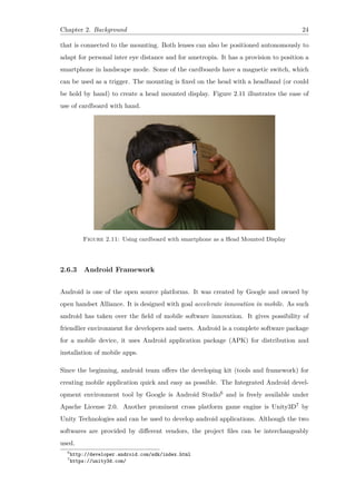
smartphones being omnipresent in everyday life are used for 3D representation most
spectacularly as a head-mounted display.
1.1 Literature Survey
In Stereo Vision, two cameras which are displaced horizontally from one another are
used to capture two views of a scene. In a manner similar to human binocular vision.
Upon comparing these two images, the lost depth information can be recovered. For the
purpose of 3D reconstruction from stereo pair, given two projections of the same point
in the world onto the two images, its 3D position can be found as the intersection of the
two projection rays. This process can be repeated for several points yielding the shape
and configuration of the objects in the scene [1]. Stereo Vision can be used with 3D
Pattern Matching and Object Tracking and is therefore used in applications such as bin
picking, surveillance, robotics, and inspection of object surfaces, height, shape, etc.
Stereo reconstruction from image pairs is a standard method for 3D acquisition of human
faces. Stereo vision has a couple of synchronized camera with known parameters and
fixed mutual positions. Depending on available imagery and accuracy requirements
the resulting 3D reconstructions may have deficits. The stereo image pair needs to be
acquired with a relatively short baseline length in order to avoid occlusions [2] e.g. When
capturing the human face if the two stereo cameras are far away the person’s nose would
occlude some portion of face in both the images, resulting in steep intersection angles of
the two view rays limiting the accuracy of depth measurement. Furthermore, in some
areas of the face the view rays are relatively tangential to the surface making surface
reconstruction more difficult. Another problem, in particular for imagery lacking spatial
resolution, is the lack of texture in some parts of faces. The unavoidable consequence of
these problems is the limited accuracy of surface reconstruction.1
The deficits of 3D stereo reconstruction can be alleviated by the use of prior knowledge.
In principle as well as from a historic viewpoint the use of prior knowledge in shape
reconstruction has a long history in craftsmanship and engineering. One can even claim
that the more limited measurement devices were in previous periods of technological
1
Depending on defined demands this is certainly true for any measurement process.](https://image.slidesharecdn.com/6bfb7267-8a6b-438d-b02e-1c853b91f5b8-160731060201/85/main-11-320.jpg)
![Chapter 1. Introduction 3
development, the more prominent the use of prior knowledge was. Only with the ad-
vent of mass measurement devices such as cameras and laser scanners the use of prior
knowledge disregarded to larger extent.2
In order to be generally usable the type of prior knowledge to be used should be rather
generic and not particularly object specific. In our example, prior knowledge about face
geometry will be provided by the same 3D model to be used for any person’s face to
be reconstructed. In the processing steps of the procedure the 3D model will first be
adapted to better represent one of the two images of a stereo pair.
The 3D model used for reconstruction is referred to as 3D Morphable Model of face.
Based on input image the model parameters are modified to fit the face image [3], the
technique is referred to as face modeling. When discussing about the prior knowledge,
the major limitation of automated technique for face modeling from single image is either
the problem of locating features in faces or the dilemma of separating realistic from non
real faces, which could never exists [4].
For the first problem, the feature location (50 to 100 points) when done manually usually
requires hours and accuracy of an expert. Human perception about faces is necessary
to compensate for variations between different faces and to ensure a valid feature point
assignment. Till date, automated feature point matching algorithms are available for
salient features like the corners of lips or the tip of nose.
In the second problem of face modeling, the human knowledge is more significant for
separation of natural (real) faces from unnatural looking faces and avoid non realistic
face results. Some application of face modeling even involves the design of completely
new natural looking face, which can occur in real world but has no actual counterpart.
Others require the handling of existing face in accordance with changes in age, sex, body
weight and race or to simply enhance the characteristics of the face. These tasks might
require plenty of time with combined efforts of an artist. The problem of non face like
structures can be solved by creating a model from real faces, which has scan of real
world human faces of different age, sex and race.
One of the tasks required in face analysis is to perform face reconstruction from input
images. Given a single face input image, a generalized face model is commonly used
to recover shape and texture via a fitting process. However, fitting the model to the
2
For instance in medieval time periods the 3D geometry of a cubical wooden box would have been
acquired by the three distance measurements of height, length and depth plus the prior knowledge that
the object of interest has a cubical shape, and not by thousands of 3D point measurements.](https://image.slidesharecdn.com/6bfb7267-8a6b-438d-b02e-1c853b91f5b8-160731060201/85/main-12-320.jpg)
![Chapter 1. Introduction 4
facial image remains a challenging problem. Many models have been proposed for this
purpose. The face models are a powerful tool of computer vision and are classified in
two groups: 2D face models and 3D face models.
The Active Appearance Model (AAM) by Cootes et al. [5] belong to the 2D group. It
models the shape and texture variations statistically. The authors in [6] when observed
the relationship between the resolution of the input image and the model, concluded
that the best fitting performance is obtained when the input image resolution is slightly
lower than the 2D model resolution.
Although AAMs exhibit promising face analysis performance, there is still a problem
that the reconstruction with AAMs fails if the in-depth rotation of the face becomes
large. Almost all the 2D-based models suffer from the same problem.
The 3D model has distinctive advantage over the 2D, in Active Appearance Models the
correlations between texture and shape are learned to generate a combined appearance
model. Where as in a 3D model, the shape of a face is clearly separated from the pose.
Its projection to the 2D is modeled by affine or perspective camera model. Also, the
use of a 3D face model allows us to model the light explicitly since the surface normals,
depth and self-occlusion information are available. The illumination model separates
light from the face appearance and is not incorporated with the texture parameters, as
it is for the case in 2D AAMs. The main advantage of 3D based models is that 3D shape
does not change under different viewpoint and so are more robust than their 2D counter
part.
The generative model in this study focuses on 3D Morphable Model (3DMM) which
were first proposed by Blanz and Vetter [4]. In 2009, Basel Face Model (BFM) [7] was
introduced which spurred the research with 3D Morphable Models. It surpassed the
existing models due to the accuracy of 3D scanners used and the quality of registration
algorithms. The multi segment BFM, along with some fitting results and metadata
can be obtained by signing a license agreement. This led to its implementation in face
recognition in video [8], and Linear Error function based Face identification by fitting
a 3DMM [9]. While the BFM provides the model, they only provide fitting result for
limited database and do not provide algorithms to implement the model to new images
[10]. This restricted its application to a closed domain.
The 3DMM attempts to recover the 3D face shape which has been lost through projec-
tion from 3D into 2D image. Given a single facial image, a 3DMM can retrieve both](https://image.slidesharecdn.com/6bfb7267-8a6b-438d-b02e-1c853b91f5b8-160731060201/85/main-13-320.jpg)
![Chapter 1. Introduction 5
intra-personal (pose, illumination) and inter-personal (3D shape, texture) via a fitting
algorithm. Furthermore, a 3DMM can be used in a productive way to create specific
faces or to generate annotated training data sets for other algorithms that covers a
variety of pose angles. Thus the 3DMM is crucial for variety of applications in Com-
puter Vision and Graphics. The application of 3DMMs include face recognition, 3D face
reconstruction, face tracking.
The so-called fitting algorithms that solve these cost functions are often very complex,
slow, and are easily trapped in local minima. These methods can be roughly classified
into two categories: first ones with linear cost functions and those with non-linear. The
algorithms falling in first category generally use only prominent facial landmarks like eye
or mouth corners to fit the shape and camera parameters, and use image pixel value to fit
color and light model [9]. The algorithms of later category consist of more complicated
cost functions applying a non-linear solver to iteratively solve for all the parameters
[8, 11, 12].
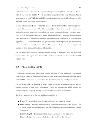
The use of 3D Visualization is standard today, but Visualization devices are still con-
trolled by standard PC and screens. Different low-cost-systems for 3D Visualization are
present as inexpensive alternatives to complex virtual reality systems such as a CAVE
or a 3D power wall. Low-cost-systems for the visualization (display and control) are
defined by the cost of the hardware not exceeding smartphones for |15000 (e 200).
Low-cost-system components such as mobile phone can be used for the stereoscopic
display of the objects. A smartphone can be used to visually inspect results of image-
based 3D reconstruction. An application (app) for an Android smartphone allowing to
view 3D point clouds could be best suited. By using a smart phone app, the device
becomes a Head Mounted Display (HMD) to create an even more immersive exploration
of the data. The inertial sensors of the phone can be used for the tracking of the
head, Since the interactive visualization should allow free movement or navigation of
the user in the 3D model. Necessary input commands must be captured and processed
using appropriate hardware, which must be sent as input data to the Visualization
software. The navigation parameters are continuous changes of the camera position and
orientation, which are defined interactively by the user.](https://image.slidesharecdn.com/6bfb7267-8a6b-438d-b02e-1c853b91f5b8-160731060201/85/main-14-320.jpg)
![Chapter 1. Introduction 6
1.2 Motivation and Objectives of the Dissertation
3D reconstruction is an ill-posed problem, various modern algorithm have been developed
to achieve this. Majority of these methods either involves multiple images as input or
a single image with some object information. we would be dealing in the combination
of two methods for human face and the accomplished object is the geometrically rich
deformed face model.
3D reconstruction of object based on measurement data from e.g.imaging sensors would
quite generally profit from the use of prior information about the object’s shape. As the
stereo reconstruction poses few deficits in the reconstruction, the prior knowledge in the
form of single image reconstruction could be used.
The use of morphable model as the basis for 3D reconstruction was introduced by Blanz
and vetter and the majority of literature regarding the morphable face models is based
on their work. Recently, 3DMMs provided by University of Surrey have been used with
regression-based methods [3] which is a leap forward in the direction of face modeling.
No significant improvement in the face modeling has been brought in it since then.
Automation in the process of single image face reconstruction has not been still achieved
because of manual landmark annotations or premarked landmark coordinates being used.
This gap has also been bridged in this work, by using the regression tree method [13]
by V. Kazemi et al. This method identifies landmark positions of faces like tip of eyes,
eyebrows, lips and Nose; which are used for fitting the morphable model to the single
face image.
The Morphable model has an advantage of giving 3D structure from a single image, but
it doesn’t conforms to the actual congruous of the face. The reason being it is based
on few landmark positions only. A geometrically more definite description of the face is
stereo reconstruction. Deformation, which is one of the crucial step of this pipeline and
obviously some of the most difficult procedure has to be carried out on the face model,
so as to result in a deformed face model. Thus concluding model holds the best of face
model and stereo model.
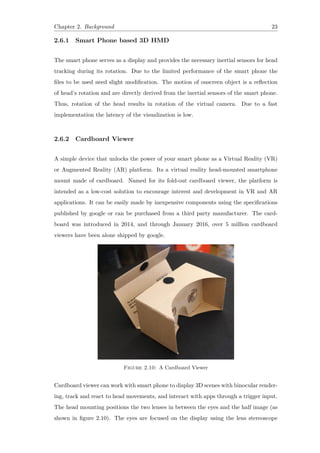
Cardboard has brought a revolution in the Virtual Reality and its depended applications
in healthcare, entertainment and scientific visualization. An economical head mounted
cardboard has changed the way 3D objects can be anticipated on a screen. Various
well known companies have developed there own Virtual Reality (VR) visualisers like](https://image.slidesharecdn.com/6bfb7267-8a6b-438d-b02e-1c853b91f5b8-160731060201/85/main-15-320.jpg)

![Chapter 2
Background
For a better understanding of the basic concepts used in this work, some prerequisites
are discussed in this chapter. The first one is Facial Point Annotation which is used for
landmarking on face image. Next section introduces the 3D morphable model with its
composition information. Texture representation uses isomap algorithm, details of which
are discussed in third section. Another reconstruction technique i.e.stereo reconstruction
is included next. Later section includes the Deformation of Face Model which is an
integral part of this thesis. The last section discusses the Visualization of the resultant
model on smartphone.
2.1 Facial Point Annotation
Detecting facial features is the problem of detecting semantic facial points in an image
such as tip of lips, eyes, mouth and boundary of face. Apart from its application in Face
reconstruction from a 3DMM, facial feature detection concerns various other research
applications which include Face Recognition of pre-learnt faces in unseen images, Face
Hallucination (synthesizing a high-resolution facial image from a lower resolution),
Face Animation (real-time animation of a graphical avatars expression based on real
facial expression).
Facial point annotation can be achieved by variety of algorithms. One of these, Cascade
based regression methods by V. Kazemi et al. uses an Ensemble of Regression Trees [13],
8](https://image.slidesharecdn.com/6bfb7267-8a6b-438d-b02e-1c853b91f5b8-160731060201/85/main-17-320.jpg)
![Chapter 2. Background 11
2.1.2 Learning each Regressor in Cascade
For training each rt, the gradient tree boosting algorithm with a sum of square error
loss is implemented [13]. Assume the training data (I1, F1), . . . , (In, Fn), where each Iq
is a face image and Fq is its conforming feature vector. The training data is created in
triplets to learn the first regression function r0 in the cascade. The triplet is made up of
face image, an initial shape estimate and the target update step, i.e. (Iπq, ˆF
(0)
q , ∆F
(0)
q )
where:
πq ∈ {1, . . . , n} (2.2)
ˆF
(0)
q ∈ {F1, . . . , Fq}/Fπq (2.3)
∆F(0)
q = Fπq − ˆF
(0)
q (2.4)
for q = 1, . . . , Q. the total of Q(= nR) triplets are taken, where R is the number of
initialization used per image Iq.
From this data the regression function ro is learnt, using gradient tree boosting with a
sum of square error loss. The training triplet is then updated to provide the new training
data (Iπq, ˆF
(1)
q , ∆F
(1)
q ), for the next regressor r1 in the cascade by setting (t = 0) in
Equation 2.1
ˆF
(1)
q = ˆF
(0)
q + rt(I, ˆF
(0)
q ) (2.5)
∆F(t+1)
q = Fπq − ˆF
(t+1)
q (2.6)
This process is iterated till a cascade of T regressors r0, r1, . . . , rT−1 are learnt which
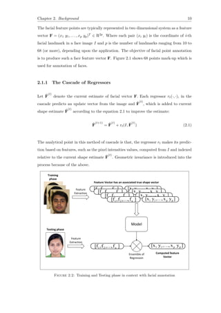
can be combined to give satisfactory level of accuracy. Figure 2.2 shows the training
and test phases of landmarking algorithm.
2.2 The Surrey Face Model
The Surrey Face Model (SFM) consists of shape and color (or so-called albedo) Principal
Component Analysis (PCA) models. PCA is a way of identifying patterns in data, and
expressing the data in a way to highlight their similarities and differences. The identified
pattern can be used to compress the data by reducing the number of dimensions, without
much loss of information.](https://image.slidesharecdn.com/6bfb7267-8a6b-438d-b02e-1c853b91f5b8-160731060201/85/main-20-320.jpg)
![Chapter 2. Background 12
SFM is available in three different resolution levels. In addition to the high resolution
models accessible via the University of Surrey2, an open source low-resolution shape-only
model is freely available on Github3, which has been used in this work. The following
sections would describe the model in detail.
2.2.1 Construction of a Face Model
The first step in the generation of model involves, collection of suitable database of
3D face scans that include shape and texture. For the robustness of the model it is
essential to be a representative of the high inter-person variability. The recorded subjects
in SFM have a diversity in skin tone and face shape to well represent multicultural
make up of many modern societies. The ideal 3D face scans only capture the intrinsic
facial characteristics, removing hair occlusions, makeup, or facial expressions and other
extraneous factors; since these are not intrinsic to the shape or texture of the face.
Figure 2.3 shows the racial distribution of all 169 faces used in model construction.
Unlike BFM, the Surrey Face model has included significant number of non-Caucasian
people to generalize the model [10]. The pie-chart in Figure 2.4 shows the age groups of
the face scans, its evident that the SFM contains more people from 20+ age category.
Figure 2.3: Racial distribution of 169
scans used to train the Surrey Face
Model.
Figure 2.4: Age groups distribution of
the 169 scans.
3dMDface4 camera system was used to capture these scans. The system consists of two
structured light projectors, 4 infrared camera and 2 RGB cameras. The infrared camera
captures the light pattern and are used to reconstruct the 3D shape. The high resolution
face texture is recorded by RGB cameras. One half of the cameras record 180° view of
the face from left side and other half from the right side. Uniform lighting condition
2
http://www.cvssp.org/faceweb/
3
https://github.com/patrikhuber/eos/blob/master/share/sfm_shape_3448.bin/
4
http://www/3dmd.com](https://image.slidesharecdn.com/6bfb7267-8a6b-438d-b02e-1c853b91f5b8-160731060201/85/main-21-320.jpg)
![Chapter 2. Background 13
are maintained to avoid shadow and specularities and ensures the model texture is
representative of face color (albedo) only and reduces the significance of the components
which are not inherent characteristics of a human face.
The most challenging task in building the model is establishing dense correspondence
across the database. Each raw face scan comprises a 3D mesh and a 2D RGB texture
map (as shown in figure 2.5). The (x, y, z) coordinates of the vertices of the 3D mesh of
the jth face scan can be concatenated into a shape vector as:
Shapej = [x1 y1 z1, . . . , xn yn zn]T
(2.7)
And similarly for the RGB values of texture map in the texture vector as:
Texturej = [R1 G1 B1, . . . , Rn Gn Bn]T
(2.8)
Figure 2.5: 3D data acquired with a 3dMDTM
sensor. Textured mesh, 3D mesh, and
texture map are shown [14].
However for each new scan the values of n (the number of shape and texture components
in a scan) will be different. In addition to it, the new face scan will not be aligned
since they are captured with different pose. This problem is solved by using Iterative
Multi-resolution Dense 3D Registration (IMDR) algorithm [15], which brings these scans
in correspondence. To establish dense correspondence among all scans, a deformable](https://image.slidesharecdn.com/6bfb7267-8a6b-438d-b02e-1c853b91f5b8-160731060201/85/main-22-320.jpg)
![Chapter 2. Background 14
reference 3D face model is used to perform a combination of local matching, global
mapping and energy-minimization.
2.2.2 3D Morphable Model
In Face reconstruction, 3D Morphable Models can be used to infer the 3D information
from a 2D image. The 3D Morphable Model is a three dimensional mesh of faces which
have been registered to a reference mesh through dense correspondence. It is required for
all the faces to be have same number of vertices in corresponding face locations. Under
these constraints a shape vector is represented by sj = [x1 y1 z1, . . . , xv yv zv]T ∈
R3v, containing the x, y and z components of the shape, and a texture vector tj =
[R1 G1 B1, . . . , Rv Gv Bv]T ∈ R3v, containing the per vertex RGB color information,
where v is the number of dense registered mesh vertices.
Principle component analysis is performed on these set of shape ˜S = [s1, . . . , sM ] ∈
R3v×M and texture ˜T = [t1, . . . , tM ] ∈ R3v×M vectors, where M is the number of
face meshes. PCA performs a basis transformation to an orthogonal coordinate system
formed by the eigenvectors Si and Ti of the shape and texture covariance matrices,
respectively in ascending order of their eigen values.
For M face meshes, PCA provides a mean face ¯s, a set of M − 1 principal components,
the ith of which is denoted by Si (also called as the eigen vector) with corresponding
variance σ2
s,i (also called as eigen value). Unique face meshes can be generated by varying
the shape parameter vector cs = [α1, . . . , αM−1]T in the equation 2.9
Smod = ¯s +
M−1∑
i=1
αiσ2
s,iSi (2.9)
Similarly the equation for texture representation can be given by Tmod = ¯t+
M−1∑
i=1
βiσ2
t,iTi
with ct = [β1, . . . , βM−1]T as the texture parameter vector.
2.3 Texture Representation
The PCA color model obtained from 3DMM is a useful illustration for the appearance
of a face. But in some case it is either desirable to use pixel color information from
image or a combination of the two. The texture (pixel color information) from the input](https://image.slidesharecdn.com/6bfb7267-8a6b-438d-b02e-1c853b91f5b8-160731060201/85/main-23-320.jpg)
![Chapter 2. Background 15
image which when remapped onto the mesh sustain all details of a face’s appearance,
while some high frequency information can be absent when the face is represented by
PCA color model only. Therefore it is desirable to use a 2D representation of the whole
face mesh that can be used to store the remapped texture. This generic representation
is created by Isomap algorithm.
2.3.1 Isomap Algorithm
The Isomap algorithm initially proposed by Tenenbaum et al. [16] is a non-linear dimen-
sionality reduction technique which focuses on retaining the geodesic distance, between
data points, measured on the data’s manifold. The geodesic distance between two points
is defined as the shortest path connecting the two points without cutting through the
surface. The algorithm is used to remove the 3rd dimension of the 3D mesh to convert
it to a flat 2D surface, while preserving the area of mesh’s triangle. Figure 2.6 depicts
the working of the algorithm diagrammatically.
(a) (b)
(c)
Figure 2.6: The Isomap Algorithm Illustration
With reference to Figure 2.6, A data set of 3D points on a spiral manifold illustrates
how the algorithm exploits geodesic distance for non-linear dimensionality reduction.
For two arbitrary points (circled on non-linear manifold (a)), their Euclidean distances](https://image.slidesharecdn.com/6bfb7267-8a6b-438d-b02e-1c853b91f5b8-160731060201/85/main-24-320.jpg)
![Chapter 2. Background 16
(blue dashed line) in the high dimensional space may not depict their intrinsic simi-
larity, as measured by geodesic distance (solid blue line) along the low-dimensionality
manifold (a). The geodesic distance can be obtained (red segments in (b)) by taking
successive Euclidean distance between neighboring points. The Isomap in (c) recovers
a 2D-embedding, that preserves geodesic distance (red line) between points, where blue
straight line approximates the true geodesic distances between points in the original
manifold.
(a) Generic Model (b) isomap dimensionality reduction
Figure 2.7: Dimensionality reduction with the isomap algorithm, the 3D model before
and after the application of isomap algorithm [14].
2.4 Stereo Reconstruction
The stereo vision setup for 3D reconstruction is the closest to the human perception of 3D
reality. The images produced from two calibrated cameras provide disparity information
(or distance) between corresponding points in the two images. The resulting “disparity
map” is used to determine the relative depths of objects in the scene [17].
The typical setup contains multiple cameras oriented in the same viewing direction with
the same axis system and projection [17]. Let us assume that the setup shown in Figure
2.8. The distance between the projection centers is called the base (b) and should be
greater than zero. The center of the left camera is located at point C1, the right one lies
at a distance b on X axis at C2. The camera constant describing the idealized camera
parameters is f and f′ respectively for left and right camera. The 3D point P in space
has coordinates (xp, yp, zp), and UL and UR are the projection of the point P on left
and right image plane.](https://image.slidesharecdn.com/6bfb7267-8a6b-438d-b02e-1c853b91f5b8-160731060201/85/main-25-320.jpg)
![Chapter 2. Background 17
Figure 2.8: Basic stereo imaging scheme: The two cameras have overlapping field of
view, the points lying in this region are observed in both the images.
2.4.1 Epipolar Geometry
Epipolar geometry describes the relations between two images. It is an outcome of the
idea that projection of a 3D point gives a 2D point on an image. The 2D point on image
and the corresponding projection center gives a 3D line. The image of this 3D line as
seen from the other camera gives a 2D line on the image. It is called epipolar line. The
matching projection point of one image lies on the epipolar line of another image.
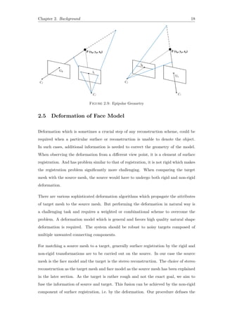
Figure 2.9 explains the epipolar geometry for stereo vision. The Projection of point P
on right image plane is at UR. The image of line joining P and UR on left image plane is
lL. The point UR has a corresponding point on this line lL. Similarly for UL the epipolar
line is lR.
If the cameras are in ideal position, the epipolar lines are parallel. These epipolar
lines are used for key point matching. Some problems, however persist: similar textures
around the epipolar line, big distance discontinuity, occluded objects [17]. Overall, stereo
imaging can be seen as robust, reliable and relatively precise technique. If using a single
stereo camera the inter calibration of camera is not required.
The epipolar relation is used to derive Fundamental Matrix which is the key to the
projection of image points back to the 3D points.](https://image.slidesharecdn.com/6bfb7267-8a6b-438d-b02e-1c853b91f5b8-160731060201/85/main-26-320.jpg)
![Chapter 2. Background 19
mesh continuity of source with the geometry of target, thus the result holds the best of
the two.
The approach differs from standard surface registration in two ways. In the first place,
natural deformation which is performed iteratively for surface registration is carried out
only once. Secondly, the requirement of optimization based on energy function is ruled
out, which significantly reduces the computational complexity.
Our deformation model is motivated by the Global Correspondence Optimization ap-
proach of H. Li et al. [18], which treats deformation as a two step approach. The choice
of routines for the deformation, differs us from global correspondence optimization. Our
work augments the parts of embedded deformation framework with a global transfor-
mation. But unlike the approach, we do not use any deformation graph and the whole
mesh is taken as a single entity.
One of the also possible ways could be treating deformation as the three dimensional
data interpolation problem. This brings us to the use of Radial Basis Function (RBF)
because of its applications in data interpolation [19], reconstruction and representation
of 3D objects [20].
A two step deformation arrangement, which addresses the local as well as global defor-
mation scheme is implemented, such that a vertex vj on the source is transformed to ˜vj
according to:
˜vj = Φlocal ◦ Φglobal(vj) (2.10)
The source mesh vertices are deformed by first applying the global deformation and then
the local deformation routine. Our approach does not require source and target to share
equal number of vertices, or to have identical connectivity. This deformation technique
is our central research contribution, details of which are discussed below.
2.5.1 Global Deformation
By Global Deformation, we mean the global change in the source, by using few anchor
points on the source mesh. These anchor points are selected by subsampling the source.
As the Radial Basis Function (RBF) have been proved successful in shape deformation
[21], it is our choice for non-rigid global deformation. RBF are means to approximate
multi variable functions by linear combinations of terms based on a single univariate](https://image.slidesharecdn.com/6bfb7267-8a6b-438d-b02e-1c853b91f5b8-160731060201/85/main-28-320.jpg)
![Chapter 2. Background 20
function. RBF interpolation sums a set of replicates of single basis function, where each
replicate is centered at a data point (called knot or center) and scaled by interpolation
condition [22].
A RBF is a real-valued function whose value depends only on the distance from the
origin, so that ϕ(x) = ϕ(∥x∥). The norm (||·||) : Rn → R) is usually Euclidean distance,
although other distance functions are also possible. Alternatively, the RBF value could
depend on the distance from some other point Xc, called a center, such that:
ϕ(x, Xc) = ϕ(∥x − Xc∥), x ∈ Rn
(2.11)
Radial basis function can be used as a weighted combination of a kernel function, which
is used to build up mesh deformation of the form:
g(x) =
N∑
c=1
λc ϕ(∥x − Xc∥) (2.12)
where the approximating function g(x) is represented as a sum of N radial basis func-
tions, each associated with a center Xc weighted by an appropriate coefficient λc. These
coefficients are calculated by considering the position of target vertices, which brings in
the influence of target in the deformation.
It should be clear from the equation 2.12, why this technique is called ”radial”, the
influence of a single data point is constant on a sphere centered at that point. The
weights λc can be estimated using the matrix methods of linear least squares, because
the approximating function is linear in the weights.
A variety of functions can be used as radial basis kernel, some of them include: Gaussian,
Thin Plate Spline, Multiquadric and Inverse Mutiquadric ([23], Appendix D). The choice
of kernel depends upon quality features required in the output. In reality there is not
yet a general characterization of what functions are suitable as RBF kernels [23].
We choose the Gaussian kernel of the form ϕ(r) = e− r2
2σ2 , where σ2 is the variance of the
normal distribution. Now we can compose the Gaussian RBF with Euclidean distance
function:
ϕi,c(x) = e−
||xi−Xc||2
2σ2 (2.13)](https://image.slidesharecdn.com/6bfb7267-8a6b-438d-b02e-1c853b91f5b8-160731060201/85/main-29-320.jpg)
![Chapter 2. Background 21
where xi is the set of vertices on source mesh. Changing the value of σ changes the shape
of the deformation function. A Gaussian RBF monotonically decreases with distance
from center Xc. A larger variance causes the function to become flatter [24].
2.5.2 Local Deformation
After the global deformation step the deviations between face model and stereo recon-
struction are locally still large. The aim of the subsequent non-rigid local deformation
is to smoothen the overshoots caused by noise or errors of the stereo reconstruction.
However, to maintain individual shape features that are only contained in the stereo
reconstruction. In other words, the local deformation step allows to transfer shape
information from the stereo reconstruction to the final face model.
The deformation of a vertex on the source is influenced by its neighboring vertices,
referring to as local deformation. The local deformation approach is derived from a
work by Sumner et al. [25] using a modified weighting scheme.
The non rigid transformation of each source vertex w.r.t. its nearest vertices on the target
is obtained by Procrustes Analysis [26]. But instead of applying non rigid transformation
of a source vertex to itself, the transformations of k-nearest neighbors is applied by a
weighted scheme. This technique creates a smooth localized deformation.
Let Bi and ti denote the components of affine transformation for all k-nearest neigh-
bors of node v. These transformations are used to transform the mesh at each node v
according to the equation:
Φlocal(v) = w0(v)[B0v + t0] +
k∑
i=1
wi(v)[Biv + ti], ∀v ∈ V (2.14)
where V denotes the set of all the source mesh vertices, k is the number of nearest neigh-
bors of node v. The w0(v) limits the influence of the node on its own transformation, B0
and t0 denote the components of affine transformation of the node. The weights wi(v)
are derived from the argument that, it must be a function of Euclidean distance of the
nearest neighbor of node v.
wi(v) = f(||vi − v||) (2.15)](https://image.slidesharecdn.com/6bfb7267-8a6b-438d-b02e-1c853b91f5b8-160731060201/85/main-30-320.jpg)


![Chapter 3
Proposed Scheme
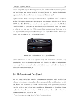
Our work uses existing single face reconstruction method by P. Huber et al. [10] on 3448
vertices shape-only Surrey 3D Morphable Face Model. It is carried out by sequentially
following Pose Estimation, Shape Fitting and Texture Extraction to generate a face
model. An improvement in the stereo reconstruction from the obtained face model by
fusing the information of the two is proposed. For the natural deformation, a combina-
tion of global and local optimization is implemented. The outcome of the deformation
is referred to as Deformed Face Model in this work. The block diagram of the complete
procedure is shown in figure 3.1
Figure 3.1: Block Diagram of proposed scheme
A face is captured by stereo camera, which gives two images. One of which is used for
single image reconstruction and the pair is used to generate the stereo reconstruction of
the face. The process begins by landmarking the face image.
26](https://image.slidesharecdn.com/6bfb7267-8a6b-438d-b02e-1c853b91f5b8-160731060201/85/main-35-320.jpg)
![Chapter 3. Proposed Scheme 27
The automated process of 3D reconstruction from an image involves some correspon-
dence between the 2D image and 3D model. These correspondences may be of different
forms depending upon the accuracy required. In our case, some feature points on Mor-
phable model are marked which uniquely identifies a human face. These points includes
corners of eyes, mouth, tip of nose and eye brows and their connecting points. These
points on image are identified by landmarking annotation algorithm.
3.1 Landmarking Annotation
The Regression based methods do not build any parametric models of shape or appear-
ance, but study the correlations between the image features to infer a facial vector. The
synthesis pipeline starts with a face detector, then the image together with the bounding
box in fed to face alignment component which return a facial vector. The face alignment
component is approached by supervised machine learning, whereby a model is trained
from a large amount of human-labeled images and can then be used for facial feature
vector (F) estimation on new face images.
3.1.1 Training data
To facilitate training, 3283 faces data collected by 300 Faces In-The-Wild Challenge
(300-W) [27] has been used. The face databases covers large variety including: different
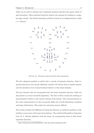
subjects, poses, illumination, occlusions. A well established landmark configuration of 68
points mark up (as shown in figure 2.1) were also available with the images. To enhance
accuracy, the annotations have been manually corrected by an expert. Additionally,
the IBUG data set consists of 135 images with highly expressive faces, difficult poses
and occlusions. The training is performed with T = 15 regressors (rt), in the cascade.
R = 20 different initializations for each training example have been used.
3.1.2 Implementing Regression Algorithm
Typically, the problem assumes an image with an annotated bounding box which sur-
rounds a face. In this case we have used an implementation of Max-Margin Object
Detection (MMOD) by D. king [28] found in the dlib c++ library. Features are ex-
tracted from the sliding boxes on the image and these are compared with the trained
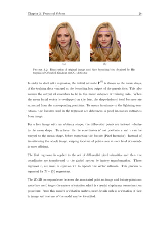
values, resulting in the bounding box as shown in Figure 3.2](https://image.slidesharecdn.com/6bfb7267-8a6b-438d-b02e-1c853b91f5b8-160731060201/85/main-36-320.jpg)
![Chapter 3. Proposed Scheme 29
Figure 3.3: The 68 point landmarks on a face Image
3.2 Pose Estimation
Given a set of 3D points on Morphable Model and corresponding 68 2D Landmark Point
(obtained in section 3.1) on a face image. The goal is to estimate the position of the
camera (or the pose of the face) in the world coordinate. An affine camera model is
assumed and Gold Standard Algorithm of Hartley & Zisserman [1] is used to compute
camera matrix P, a 3 × 4 matrix such that xi = PXi for a subset of 68 points.
First, the labeled 2D Landmark Points in the face image xi ∈ R2 and the corresponding
3D model points Xi ∈ R3 are represented in homogeneous coordinate by xi ∈ P2 and
Xi ∈ P3 respectively. Then the points are normalized by similarity transform that
translate the centroids of the point set to the respective origin and scale them so that
the Root-Mean-Square distance from their origin is
√
2 for 2D landmark points and
√
3
for model points. This makes the further algorithm invariant of similarity transform and
also nullify the effect of arbitrary position of origin in the two spaces.
˜xi = Txi, with T ∈ R3×3
(3.1)
˜Xi = UXi, with U ∈ R4×4
(3.2)
The similarity transform T and U can be obtained by equations 3.3 and 3.4. Where the
letter s and t are used to denote scaling and translation respectively in the subscript
direction.
T =
sx 0 −tx
0 sy −ty
0 0 1
(3.3)](https://image.slidesharecdn.com/6bfb7267-8a6b-438d-b02e-1c853b91f5b8-160731060201/85/main-38-320.jpg)
![Chapter 3. Proposed Scheme 30
U =
s′
x 0 0 −t′
x
0 s′
y 0 −t′
y
0 0 s′
z −t′
z
0 0 0 1
(3.4)
Now for the 2D point transformed point ˜xi = (˜ui, ˜vi, ˜wi), each correspondence between
˜xi ↔ ˜Xi gives the relation:
0T
− ˜wi
˜X
T
i ˜vi
˜X
T
i
˜wi
˜X
T
i 0T
−˜ui
˜X
T
i
−˜vi
˜X
T
i ˜uiXT ˜0
T
i
˜P
1
˜P
2
˜P
3
= 0 (3.5)
where each ˜P
iT
is a 4-vector, which is the i-th row of camera matrix ˜P. Although
in the matrix relation 3.5 there are three equations, but only two of them are linearly
independent (since the third row is a linear combination of first two). Thus each 2D-3D
point correspondence gives two equations in the entries of ˜P. Rewriting the equation
3.5 with ˜xi = (˜xi, ˜yi, 1) implies ˜xi = ˜ui
˜wi
, ˜yi = ˜vi
˜wi
:
0T
− ˜X
T
i ˜yi
˜X
T
i
˜X
T
i 0T
−˜xi
˜X
T
i
˜P
1
˜P
2
˜P
3
= 0 (3.6)
solving equation 3.6 for affine camera matrix i.e. with ˜P
3
= [0 0 0 1]T , we get
0T ˜P
1
− ˜X
T
i
˜P
2
+ ˜yi
˜X
T
i
˜P
3
˜X
T
i
˜P
1
+ 0T ˜P
2
− ˜xi
˜X
T
i
˜P
3
= 0
0T ˜P
1
+ ˜X
T
i
˜P
2
− ˜yi
˜X
T
i
˜P
1
+ 0T ˜P
2
− ˜xi
= 0
0T ˜P
1
+ ˜X
T
i
˜P
2
˜X
T
i
˜P
1
+ 0T ˜P
2
=
˜yi
˜xi
0T ˜X
T
i
˜X
T
i 0T
˜P
1
˜P
2
=
˜yi
˜xi
(3.7)](https://image.slidesharecdn.com/6bfb7267-8a6b-438d-b02e-1c853b91f5b8-160731060201/85/main-39-320.jpg)
![Chapter 3. Proposed Scheme 31
Each correspondence of ˜xi and ˜Xi contributes to equation 3.7 which are stacked into
a 2n × 8 matrix equation A8p8 = b, where p8 is the 8-vector containing the first two
rows of ˜P. The affine camera matrix has 8 degrees of freedom (8 unknowns) for which
we require four equations (n = 4), each solving for two unknowns.
In order to reduce the observation error, the actual number of correspondences is more
than four, which results in an non square matrix A8 of size m×n, m > n, so the solution
is obtained by taking pseudo-inverse of A8 denoted by A+
8 .
p8 = A+
8 b (3.8)
Horizontal concatenation of three vectors ˜P
1T
, ˜P
2T
and ˜P
3T
(= [0 0 0 1]) gives the nor-
malized affine camera matrix ˜P. The actual camera matrix by is obtained by performing
de-normalization step by transformation matrices:
P = T−1 ˜PU (3.9)
Once the pose has been estimated, now the task is to reach to the actual model shape
which resembles to the image. This is accomplished by estimation of shape parameter
vector, which depends upon the landmark positions. These shape parameter vector
when used in the 3DMM gives the Face Model corresponding to the face. Subsequently,
the camera orientation matrix along with the Isomap algorithm is used for texture map
extraction from the single image.
3.3 Shape Fitting
The shape parameters are recovered using a probabilistic approach, which maximizes
the posterior probability. The aim is to find the most likely shape vector cs given
an observation of N 2D feature landmark points in homogeneous coordinates: y =
[x1 y1 1, ..., xN yN 1]T
and taking into consideration the model prior. From Baye’s rule
we can state the posterior probability of variance normalized shape parameter (cs) w.r.t.
y as
P(cs|y) = v · P(y|cs) · P(cs) (3.10)
where v = (
∫
P(y|c′
s) · P(c′
s)dc′
s)−1 is a constant factor. The coefficients of shape pa-
rameters are normally distributed with zero mean and unit variance, i.e. c′
s ∼ N(0,IN),](https://image.slidesharecdn.com/6bfb7267-8a6b-438d-b02e-1c853b91f5b8-160731060201/85/main-40-320.jpg)
![Chapter 3. Proposed Scheme 32
so the probability of observing a given cs is
P(cs) = vc · e
−1
2
||cs||2
(3.11)
where vc = (2π)−m′/2 . The probability of observing y for a given cs is given by:
P(y|cs) =
3N∏
i=1
vN · e
− 1
2σ2
2D,i
[ymodel2D,i−yi]2
(3.12)
Here, ymodel2D,i are the homogeneous coordinates of the 3D feature points (marked on
model) projected to 2D, defined as follows:
A matrix ˆS ∈ R3N×m−1 is constructed by sub-selecting the rows of eigenvalues S associ-
ated with N landmark points. In order to give matrix a homogeneous shape, the matrix
is further modified by inserting a row of zeros after third row of S, resulting in matrix
ˆSh ∈ R4N×m−1. Now a block diagonal matrix C ∈ R3N×4N is formed, in which the the
camera matrix is placed on the diagonals:
C =
P . . . 0
...
...
...
0 . . . P
(3.13)
Finally the 2D point obtained by projecting the 3D model point given by
ymodel2D,i = Ci · (ˆShdiag(σ2
s )cs + ¯v) (3.14)
where Ci is the ith row of C.
Substituting equation 3.11 and 3.12 in the Baye’s rule equation 3.10, the conditional
probability is given by
P(cs|y) = v · vl
N · vc · e
−
∑3N
i=1
[ymodel2D,i−yi]2
2σ2
2D,i · e−1
2
||cs||2
= v · vl
N · vc · e
−1
2
[
∑3N
i=1
[ymodel2D,i−yi]2
σ2
2D,i
+||cs||2
]
which can be maximized by minimizing the exponent:
E = −2 · logP(cs|y) =
3N∑
i=1
[ymodel2D,i − yi]2
σ2
2D,i
+ ||cs||2
+ constant (3.15)](https://image.slidesharecdn.com/6bfb7267-8a6b-438d-b02e-1c853b91f5b8-160731060201/85/main-41-320.jpg)
![Chapter 3. Proposed Scheme 33
Substituting the statistical model equation 3.14 with a = diag(σ2
s )cs into the equation
3.15:
E =
3N∑
i=1
[Ci · ˆSha + Ci · ¯v − yi]2
σ2
2D,i
+ ||cs||2
E =
3N∑
i=1
[Ci · ˆSha + Ci · ¯v]2 − 2[Ci · ˆSha + Ci · ¯v]yi + y2
i
σ2
2D,i
+ ||cs||2
E =
3N∑
i=1
(Ci · ˆSha)2 + (Ci · ¯v)2 + 2Ci · ˆShaCi · ¯v − 2Ci · ˆShayi − 2Ci · ¯vyi + y2
i
σ2
2D,i
+ ||cs||2
For clarity, using Ri = Ci · ˆSh , ki = Ci · ¯v and cs = a
diag(σ2
s,i)
in the above equation
E =
3N∑
i=1
(Ria)2 + k2
i + 2Riaki − 2Riayi − 2kiyi + y2
i
σ2
2D,i
+ ∥
a
diag(σ2
s,i)
∥2
(3.16)
The error function E has to be minimized so differentiating with respect to a and set
the derivative to zero.
▽E =
3N∑
i=1
2RT
i Ria + 2RT
i ki − 2RT
i yi
σ2
2D,i
+
2a
[diag(σ2
s,i)]2
= 0
3N∑
i=1
RT
i Ria + kiRT
i − yiRT
i
σ2
2D,i
+
cs
diag(σ2
s,i)
= 0 (3.17)
Since the system of equation has to be solved for cs instead of a, so multiplying the
equation by diag(σ2
s,i), and using Qi = Ridiag(σ2
s,i), we obtain:
3N∑
i=1
diag(σ2
s,i)RT
i Ricsdiag(σ2
s,i) + kidiag(σ2
s,i)RT
i − yidiag(σ2
s,i)RT
i
σ2
2D,i
+ cs = 0
3N∑
i=1
QT
i Qics + kiQT
i − yiQT
i
σ2
2D,i
+ cs = 0
3N∑
i=1
QT
i Qics
σ2
2D,i
+ cs =
3N∑
i=1
yiQT
i
σ2
2D,i
−
3N∑
i=1
kiQT
i
σ2
2D,i
(3.18)
For simplicity we set:
T1 =
3N∑
i=1
QT
i Qi
σ2
2D,i
and T2 =
3N∑
i=1
yiQT
i
σ2
2D,i
−
3N∑
i=1
kiQT
i
σ2
2D,i](https://image.slidesharecdn.com/6bfb7267-8a6b-438d-b02e-1c853b91f5b8-160731060201/85/main-42-320.jpg)
![Chapter 3. Proposed Scheme 34
and obtain the following equation: T1cs + cs = T2. This can be solved by applying a
cholesky decomposition to T1:
using T1 = MT
M =⇒ MT
Mcs + cs = T2 (3.19)
Decomposing M with Singular Value Decomposition, M = UWVT
, we get:
(UWVT
)T
UWVT
cs + cs = T2
VWUT
UWVT
cs + cs = T2 (3.20)
since U is orthogonal in all columns i with wi ̸= 0, and multiplying by VT
VT
VW2
VT
cs + VT
cs = VT
T2 (3.21)
diag(wi + 1)VT
cs = VT
T2 (3.22)
cs = [diag(wi + 1)VT
]−1
VT
T2 (3.23)
Hence, using only a series of matrix multiplications, we are able to recover the maximum
likelihood of shape estimate vector cs given the location of 2D projected feature points
and projection matrix.
(a) (b)
Figure 3.4: Face image and its obtained shape Model
3.4 Texture Extraction from Image
A Texture Extraction methodology has to be implemented to have the option of using
the original image texture instead of texture reconstruction from the color morphable
model. The input to the process is the face image and camera matrix, hence it has to](https://image.slidesharecdn.com/6bfb7267-8a6b-438d-b02e-1c853b91f5b8-160731060201/85/main-43-320.jpg)
![Chapter 3. Proposed Scheme 35
be carried out after pose estimation. When carried out after shape fitting, the fitted
shape can be used for precise texture element extraction. After the matching process is
completed, the mesh triangles of optimized morphable model are projected to the image
plane using isomap algorithm and camera matrix.
When the model is projected on image, the triangles with normal > 90◦ are not visible
on image. If a triangle is visible in the image, the RGB values of the pixels of the
triangle are taken from the input image and copied to the location that corresponds to
that same triangle in the newly created texture map. In the iso texture map a fourth
quantity called alpha value is added which describes the visibility of a triangle, where
the value α is given by α = 255 × normal angle. Using the normal values of optimized
model and the z-buffer algorithm, these triangles are tested for visibility.
The texture map algorithm by P. Huber et al. [10] is efficient in evaluating the texture
components from the image but it produces holes on some positions, as observed in
Figure 3.5 (a). This holes in the texture map can be cleared by using a 3 × 3 averaging
filter, without considering the holes. The filtering is only applied in the mask area
specified by isomap algorithm as shown in figure 2.7 (b). The continuous texture can be
observed in Figure 3.5 (b).
(a) (b)
Figure 3.5: The texture maps before and after the application of averaging filter.
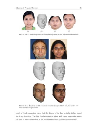
A complete combination of shape model and texture representation on a single image
is shown in Figure 3.6, the combination of shape and texture as shown in 3.6 (d) is the
resultant face model.
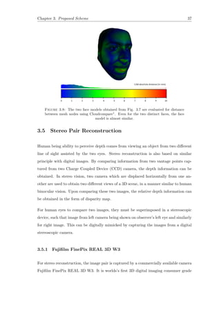
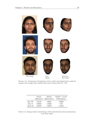
The Figure 3.7 shows two face models side by side in a comparative way. The face
model in the last row look quite identical to each other but not to the respective images.
We can observe the aspect ratio of the model, which is quite different in images. The
observation is analytically supported by the face model comparison in Fig. 3.8. The](https://image.slidesharecdn.com/6bfb7267-8a6b-438d-b02e-1c853b91f5b8-160731060201/85/main-44-320.jpg)
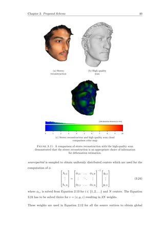
![Chapter 3. Proposed Scheme 39
(a) Left Camera Image (b) Right Camera Image
(c) Stereo Reconstruction
Figure 3.10: Images obtained from stereo camera and the surface reconstruction
obtained from the images.
For the purpose of deformation, the face model is aligned with the its stereo recon-
struction by rigid Iterative Closest Point (ICP) algorithm [29]. In the two step non-rigid
deformation, the first stage of global deformation is carried out by computing the weights
λc. The weights can be estimated using inverse matrix multiplication, because the global
deformation function in Equation 2.12 is linear in the weights. So the equation for com-
puting weights can be roughly written as λ = ϕ−1g.
Generally, all source vertices have a nearest correspondence on the target. But if the
target mesh is incomplete or partial, some of these correspondences may be wrong. For
instance, assume a source vertex having a nearest neighbor inside a hole region of the
target would now have a correspondence at the boundary vertex of the hole. Let there
be a set of all these source vertices which correspond to border vertices on the target.
A large portion of this set originates from wrong correspondences, which is why this set
is excluded from the source nodes further considered. The remaining (valid) nodes are
called sourcepartial in the following.
Target correspondences of the sourcepartial vertices contribute to the matrix g. The](https://image.slidesharecdn.com/6bfb7267-8a6b-438d-b02e-1c853b91f5b8-160731060201/85/main-48-320.jpg)

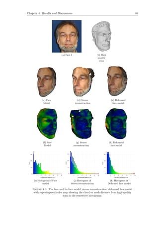
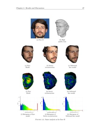
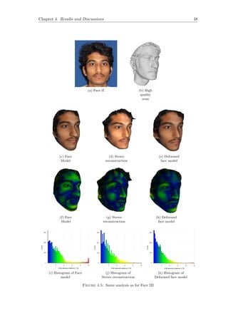
![Chapter 4. Results and Discussions 44
4.2 Qualitative Analysis
Figure 4.1 shows the results after adapting stereo reconstruction to the morphable model.
The correct difference in the aspect ratio of two face models depicts the accuracy visually.
Deformed Face model is visibly more identical to the image as compared to the face
model.
Figure 4.1: Deformed face model for faces in Fig. 3.7
In order to have a fair comparison, the results of face reconstruction from single image
and from our method is mentioned in Figure 4.2. Our method depicts the face roundness
near the beard in a proper form. The nose which was earlier bigger in face model is
appropriate in the deformed face model. The cheeks in the deformed face model are more
flat, which obeys the shape information from the stereo reconstruction. Qualitatively,
the deformed face model which is obtained by adapting stereo reconstruction to the
face model is a more accurate 3D face description. The results are also supported by
quantitative analysis, i.e. comparing the various stages of reconstruction with the High
quality face scan.
(a) Face Image (b) Face model
obtained by P. Huber
et al. [10]
(c) Deformed
model by our
approach
Figure 4.2: Comparison of Face Model with Deformed Face Model](https://image.slidesharecdn.com/6bfb7267-8a6b-438d-b02e-1c853b91f5b8-160731060201/85/main-53-320.jpg)


![Bibliography
[1] R. I. Hartley and A. Zisserman, Multiple View Geometry in Computer Vision.
Cambridge University Press, ISBN: 052162304, first ed., 2000.
[2] F. Bellocchio, N. A. Borghese, S. Ferrari, and V. Piuri, 3D Surface Reconstruction:
Multi-Scale Hierarchical Approaches. Springer Science & Business Media, 2012.
[3] P. Huber, Z.-H. Feng, W. Christmas, J. Kittler, and M. Rätsch, “Fitting 3D mor-
phable models using local features,” arXiv preprint arXiv:1503.02330, 2015.
[4] V. Blanz and T. Vetter, “A morphable model for the synthesis of 3D faces,” in
Proceedings of the 26th annual conference on Computer graphics and interactive
techniques, pp. 187–194, ACM Press/Addison-Wesley Publishing Co., 1999.
[5] T. F. Cootes, G. J. Edwards, and C. J. Taylor, “Active appearance models,” IEEE
Transactions on Pattern Analysis & Machine Intelligence, no. 6, pp. 681–685, 2001.
[6] X. Liu, P. H. Tu, and F. W. Wheeler, “Face model fitting on low resolution images,”
in BMVC, vol. 6, pp. 1079–1088, 2006.
[7] P. Paysan, R. Knothe, B. Amberg, S. Romdhani, and T. Vetter, “A 3D face model
for pose and illumination invariant face recognition,” in Advanced Video and Sig-
nal Based Surveillance, 2009. AVSS’09. Sixth IEEE International Conference On,
pp. 296–301, IEEE, 2009.
[8] R. van Rootseler, L. Spreeuwers, and R. Veldhuis, “Using 3D morphable mod-
els for face recognition in video,” in Proceedings of the 33rd WIC Symposium on
Information Theory in the Benelux, (Enschede, the Netherlands), pp. 235–242,
Werkgemeenschap voor Informatie- en Communicatietheorie, WIC, May 2012.
55](https://image.slidesharecdn.com/6bfb7267-8a6b-438d-b02e-1c853b91f5b8-160731060201/85/main-64-320.jpg)
![Bibliography 56
[9] S. Romdhani, V. Blanz, and T. Vetter, “Face identification by fitting a 3D mor-
phable model using linear shape and texture error functions,” in Computer Vision—
ECCV 2002, pp. 3–19, Springer, 2002.
[10] P. Huber, G. Hu, R. Tena, P. Mortazavian, W. P. Koppen, W. Christmas,
M. Rätsch, and J. Kittler, “A multiresolution 3D morphable face model and fitting
framework,” in 11th International Joint Conference on Computer Vision, Imaging
and Computer Graphics Theory and Applications, February 2016.
[11] S. Romdhani and T. Vetter, “Estimating 3D shape and texture using pixel intensity,
edges, specular highlights, texture constraints and a prior,” in Computer Vision and
Pattern Recognition, 2005. CVPR 2005. IEEE Computer Society Conference on,
vol. 2, pp. 986–993, IEEE, 2005.
[12] J. R. Tena, R. S. Smith, M. Hamouz, J. Kittler, A. Hilton, and J. Illingworth, “2D
face pose normalisation using a 3D morphable model,” in Advanced Video and Signal
Based Surveillance, 2007. AVSS 2007. IEEE Conference on, pp. 51–56, IEEE, 2007.
[13] V. Kazemi and J. Sullivan, “One millisecond face alignment with an ensemble of
regression trees,” in Computer Vision and Pattern Recognition (CVPR), 2014 IEEE
Conference on, pp. 1867–1874, IEEE, 2014.
[14] J. Tena Rodríguez, 3D Face Modelling for 2D+3D Face Recognition. PhD thesis,
University of Surrey, 2007.
[15] J. R. Tena, M. Hamouz, A. Hilton, and J. Illingworth, “A validated method for
dense non-rigid 3D face registration,” in Video and Signal Based Surveillance, 2006.
AVSS’06. IEEE International Conference on, pp. 81–81, IEEE, 2006.
[16] J. B. Tenenbaum, V. De Silva, and J. C. Langford, “A global geometric framework
for nonlinear dimensionality reduction,” Science, vol. 290, no. 5500, pp. 2319–2323,
2000.
[17] P. Zemcik, M. Spanel, P. Krsek, and M. Richter, “Methods of 3D object shape
acquisition,” 3-D Surface Geometry and Reconstruction: Developing Concepts and
Applications: Developing Concepts and Applications, p. 1, 2012.
[18] H. Li, R. W. Sumner, and M. Pauly, “Global correspondence optimization for non-
rigid registration of depth scans,” in Computer graphics forum, vol. 27, pp. 1421–
1430, Wiley Online Library, 2008.](https://image.slidesharecdn.com/6bfb7267-8a6b-438d-b02e-1c853b91f5b8-160731060201/85/main-65-320.jpg)
![Bibliography 57
[19] K. Anjyo and J. Lewis, “RBF interpolation and gaussian process regression through
an rkhs formulation,” Journal of Math-for-Industry, vol. 3, no. 6, pp. 63–71, 2011.
[20] J. C. Carr, R. K. Beatson, J. B. Cherrie, T. J. Mitchell, W. R. Fright, B. C.
McCallum, and T. R. Evans, “Reconstruction and representation of 3D objects with
radial basis functions,” in Proceedings of the 28th annual conference on Computer
graphics and interactive techniques, pp. 67–76, ACM, 2001.
[21] Z. Levi and D. Levin, “Shape deformation via interior rbf,” Visualization and Com-
puter Graphics, IEEE Transactions on, vol. 20, no. 7, pp. 1062–1075, 2014.
[22] K. Anjyo, J. P. Lewis, and F. Pighin, “Scattered data interpolation for computer
graphics,” in ACM SIGGRAPH 2014 Courses, p. 27, ACM, 2014.
[23] G. E. Fasshauer, Meshfree approximation methods with MATLAB, vol. 6. World
Scientific, 2007.
[24] M. D. Buhmann, “Radial basis functions: theory and implementations,” Cambridge
monographs on applied and computational mathematics, vol. 12, pp. 147–165, 2004.
[25] R. W. Sumner, J. Schmid, and M. Pauly, “Embedded deformation for shape ma-
nipulation,” ACM Transactions on Graphics (TOG), vol. 26, no. 3, p. 80, 2007.
[26] D. G. Kendall, “A survey of the statistical theory of shape,” Statistical Science,
pp. 87–99, 1989.
[27] C. Sagonas, G. Tzimiropoulos, S. Zafeiriou, and M. Pantic, “300 faces in-the-wild
challenge: The first facial landmark localization challenge,” in Proceedings of the
IEEE International Conference on Computer Vision Workshops, pp. 397–403, 2013.
[28] D. E. King, “Max-margin object detection,” arXiv preprint arXiv:1502.00046, 2015.
[29] P. J. Besl and H. D. McKay, “A method for registration of 3-D shapes,” IEEE
Transactions on Pattern Analysis and Machine Intelligence, vol. 14, pp. 239–256,
Feb 1992.](https://image.slidesharecdn.com/6bfb7267-8a6b-438d-b02e-1c853b91f5b8-160731060201/85/main-66-320.jpg)

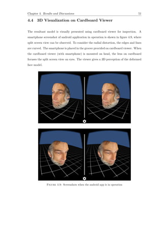
This document describes a dissertation that aims to improve 3D stereo reconstruction of human faces by combining it with a generic morphable face model. The dissertation first discusses background topics like facial landmark annotation, 3D morphable face models, texture representation, stereo reconstruction and face model deformation. It then describes the proposed scheme which involves steps like landmark annotation, pose estimation, shape fitting, texture extraction, stereo reconstruction from image pairs and deformation of the face model. The results show that fusing the stereo reconstruction with a single image reconstruction using a morphable model leads to a more accurate 3D face model compared to using either method alone. Finally, the deformed face model is visualized on a smartphone using a cardboard viewer.