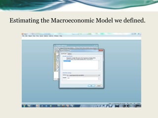
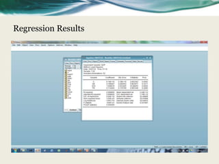
1. Time Series Modelling using Eviews
2. Macroeconomic Modelling using Eviews
3. Macroeconometrics using Eviews


                                                     By: Muhammad Anees
                                                 Saturday, October 27, 2012
                          Learn Econometrics, Applied Statistics, Stata, SPSS,
                                                   Eviews, R and Matlab on
                                    http://elearning.aneconomist.com
Plan of the Session

•   Some Theoretical Aspects?


•   Modelling the Systems


•   Proceeding with Eviews (Eviews 7)
Macroeconomic Models
Examples
Flow of Modelling Strategy
It depicts the flow of identifying a model for the system
Our Todays Strategy

Identify a simple Model and Estimate the Model using
Eviews 7 using the given data for Pakistan

Second Session Will continue from here and will develop
a more technical model


                   The                       Eviews
   Model         Variable       Data
                    s                         Steps
Macroeconomic Model of Pakistan
Economy: The real Sector
•   The sample Modelling of Pakistan’s real economy
    will develop the relationship between GDP, E , I,
    GVA, (X-M: BOP or Trade Balance)?
•   The model we will elaborate and estimate is GDP =
    E + I + GVA+(X – M)?
•   Known issues?
    o   The relation between the macroeconomic variable poses
        some technical, Econometric challenges to estimate.
        And read some literature on what are these challenges if
        estimated using simple Regression or Vector
        Autoregressive Models/Cointegrated Relations?
•   These issues are for the next sessions, please
    wait!!!!
The data

•   We have extracted a sample dataset from the databank of World bank
    which is available from data.worldbank.org
•   The variables included are:
    o   GDP:
    o   E:
    o   I:
    o   GVA
    o   X-M
•   The data is from variables (gdp       ge inv      gva      imp      exp)
•   We take log of each series so when the log difference is used, it will show
    growth rates of the series/variable
Econometric Techniques
•   OLS
    o   Please read the first section of Growth Models reading which will explain each step we proceed
        to run the regression using OLS and related tests.
•   Unit Root
    o   We will need these types of tests when we need to run a regression model using time series data
    o   As we estimate the model (any other model can be used equally) using OLS, so the results will
        be SPURIOUS/not be consistent.
    o   In this case, we need to estimate the stationarity of the series. If series are stationary, then we
        will be using OLS and may/may not include the trend/time variable
    o   If the series are not stationary then we will test for whether each series is uniformly/same
        integrated. Which means they become stationary at the same level of differencing.
    o   Detailed discussion on these and the following contents will be provided tomorrow. This is
        introduced here to convince you that we can not rely on the OLS estimates of our model using
        time series data.
•   Cointegration
•   VAR
•   VECM
Appendix

•   Estimating the Model using OLS
•   Testing for Issues in the estimated Models
•   Some Econometric tests which could be used to determine whether the
    model estimated is best fitted
•   Why we need to use alternative/Time Series regression Models? Read
    the Unit Roots, VAR and Cointegration Testing topics from the given
    reading material. We will improve our current model in second session.
•   Contact information: Please use only moodle@aneconomist.com for
    discussion regarding these contents. This email is specific to course
    related discussions.
Please read the notes below for details
Workfile Dialague to create workfile
New Workfile where data will be imported.
Import Wizard
Import Wizard: Data Specification
Dated Workfile with Complete dataset
Estimating the Macroeconomic Model we defined.
Regression Results
OLS Examples where it is Spurious
What Then if OLS is Spurious

•   If we use most of the Time Series data for running OLS, then results
    are spurious if the Data is Not Stationary/Unit Root. Now how to
    test Unit Roots. Let us what we can do using Eviews.
Unit Roots Testing
Unit Roots Testing
Unit Root Results
Unit Root test with First Difference
Unit Roots and Order of Integration

•   If we find that all the series are unit root or stationary then decide as
    following:
    o   All Series are not Unit Root or say they are stationary in Levels, then these are
        called Integrated of Order Zero and termed as I(0)
    o   All the series are Unit Root at Levels and Stationary at First Difference then
        The are Integrated of Order One or I(1)
    o   All the series are unit root even at First Differences but Stationary at Second
        Differences then These are Integrated of Order Two or I(2).
    o   And Hence On…
    o   We proceed in the same lines and once the Integration is determined, then we
        can test whether they are Co-Integrated. This is for tomorrow along with
        Theory, Practice and Issues.
We have learn Step by Step
Outcome of Todays Session

•   We hope to know now:
•   Modelling any Macroeconomic Scenario
•   Estimate the using Basic regression and test for whether regression
    is Spurious
•   When Spurious how to proceed with further our model estimation.
•   Thanks for your attendance.
•   Please email any confusion regarding initiating your modelling
    strategy.
•   Also please read the suggested contents so we are confident for
    tomorrow session.

Macroeconomic modelling

  • 1.
    1. Time SeriesModelling using Eviews 2. Macroeconomic Modelling using Eviews 3. Macroeconometrics using Eviews By: Muhammad Anees Saturday, October 27, 2012 Learn Econometrics, Applied Statistics, Stata, SPSS, Eviews, R and Matlab on http://elearning.aneconomist.com
  • 2.
    Plan of theSession • Some Theoretical Aspects? • Modelling the Systems • Proceeding with Eviews (Eviews 7)
  • 3.
  • 4.
  • 5.
    Flow of ModellingStrategy It depicts the flow of identifying a model for the system
  • 6.
    Our Todays Strategy Identifya simple Model and Estimate the Model using Eviews 7 using the given data for Pakistan Second Session Will continue from here and will develop a more technical model The Eviews Model Variable Data s Steps
  • 7.
    Macroeconomic Model ofPakistan Economy: The real Sector • The sample Modelling of Pakistan’s real economy will develop the relationship between GDP, E , I, GVA, (X-M: BOP or Trade Balance)? • The model we will elaborate and estimate is GDP = E + I + GVA+(X – M)? • Known issues? o The relation between the macroeconomic variable poses some technical, Econometric challenges to estimate. And read some literature on what are these challenges if estimated using simple Regression or Vector Autoregressive Models/Cointegrated Relations? • These issues are for the next sessions, please wait!!!!
  • 8.
    The data • We have extracted a sample dataset from the databank of World bank which is available from data.worldbank.org • The variables included are: o GDP: o E: o I: o GVA o X-M • The data is from variables (gdp ge inv gva imp exp) • We take log of each series so when the log difference is used, it will show growth rates of the series/variable
  • 9.
    Econometric Techniques • OLS o Please read the first section of Growth Models reading which will explain each step we proceed to run the regression using OLS and related tests. • Unit Root o We will need these types of tests when we need to run a regression model using time series data o As we estimate the model (any other model can be used equally) using OLS, so the results will be SPURIOUS/not be consistent. o In this case, we need to estimate the stationarity of the series. If series are stationary, then we will be using OLS and may/may not include the trend/time variable o If the series are not stationary then we will test for whether each series is uniformly/same integrated. Which means they become stationary at the same level of differencing. o Detailed discussion on these and the following contents will be provided tomorrow. This is introduced here to convince you that we can not rely on the OLS estimates of our model using time series data. • Cointegration • VAR • VECM
  • 10.
    Appendix • Estimating the Model using OLS • Testing for Issues in the estimated Models • Some Econometric tests which could be used to determine whether the model estimated is best fitted • Why we need to use alternative/Time Series regression Models? Read the Unit Roots, VAR and Cointegration Testing topics from the given reading material. We will improve our current model in second session. • Contact information: Please use only moodle@aneconomist.com for discussion regarding these contents. This email is specific to course related discussions.
  • 11.
    Please read thenotes below for details
  • 12.
    Workfile Dialague tocreate workfile
  • 13.
    New Workfile wheredata will be imported.
  • 14.
  • 15.
    Import Wizard: DataSpecification
  • 17.
    Dated Workfile withComplete dataset
  • 18.
  • 19.
  • 20.
    OLS Examples whereit is Spurious
  • 21.
    What Then ifOLS is Spurious • If we use most of the Time Series data for running OLS, then results are spurious if the Data is Not Stationary/Unit Root. Now how to test Unit Roots. Let us what we can do using Eviews.
  • 22.
  • 23.
  • 24.
  • 25.
    Unit Root testwith First Difference
  • 26.
    Unit Roots andOrder of Integration • If we find that all the series are unit root or stationary then decide as following: o All Series are not Unit Root or say they are stationary in Levels, then these are called Integrated of Order Zero and termed as I(0) o All the series are Unit Root at Levels and Stationary at First Difference then The are Integrated of Order One or I(1) o All the series are unit root even at First Differences but Stationary at Second Differences then These are Integrated of Order Two or I(2). o And Hence On… o We proceed in the same lines and once the Integration is determined, then we can test whether they are Co-Integrated. This is for tomorrow along with Theory, Practice and Issues.
  • 27.
    We have learnStep by Step
  • 28.
    Outcome of TodaysSession • We hope to know now: • Modelling any Macroeconomic Scenario • Estimate the using Basic regression and test for whether regression is Spurious • When Spurious how to proceed with further our model estimation.
  • 29.
    Thanks for your attendance. • Please email any confusion regarding initiating your modelling strategy. • Also please read the suggested contents so we are confident for tomorrow session.

Editor's Notes

  • #12 This screen shows how we would create a work file and then save it for the session so we use it.The screen leads you to:Click FileClick NewClick WorkfileThe you will get the next screen in next slide
  • #13 When you click on the Workfile Structure Type, you need to select the undated series as we are not sure of the number of data. If you are sure of the number of observations and variable in the imported excel file, then select a relevant option. We select undated then type 1 in the Date Specification. We get an opened Workfile as seen on the next slide
  • #15 Now click on File, Click on ImportClick on Import Data FileFollow the onscreen dialogue and locate the data fileOnce opened, you will see the following screen on next slide
  • #16 Note that we need to redefine the structure of data as we earlier created new workfile with 1 observation. Hence follow the above screen and click Next and then Next. Once the process complete, a new box will appear where Next button will disappear and Finish will be Visible. Please click Finish. You will get the screen on next slide.
  • #17 Now click Yes so re-define the data structure in the workfile which we created undated. You will get the workfile change to the screen in next slide.
  • #18 After successfully importing the file, we have to save the workfile as we wish. I will name it miltonfirstsession so I remember what I did in your sessions. You can name it as you wish.
  • #19 We have variables gdp, gva, ge,exp (exp01 here) and imp in the data. We do not have exp-imp so we first generate series tr which is equal to exp01-imp where. Go to Quick, generate series and type tr=exp01-impNow we have the required data. We run the OLS here to estimate the model defined. Note this estimation is just to see the signs of the variables in the model. Now click first gdp, then press CTRL and click on each c, gva, ge and tr one by one. You can right click then on the selected series and click on As Equation. You will get the dialogue box as given on the Next Slide. You can get to this box from Menu bar Clicking Quick, Click on Estimate Equation and then type the series in sequence as gdp c gegva tr.This will result in the next slide.
  • #20 Now read the Given Growth Models and Read the Contents after the Regression from Pages: 27-29 and let us discuss any questions regarding these sections tomorrow.
  • #21 Now looking into these examples will you know what is meant by Spurious?
  • #23 Please see the Chapter on Time Series Analysis in the Ebook by Baltagi. We can test for the presence of Unit Roots following the Steps:Click On Quick from Menu BarClick on Series StatisticsClick on Unit Roots TestsYou will see the Box/Picture aboveType the Name of Any Series like gdpClick on OKThe follow the Steps in Next Slides
  • #24 Once from previous Screen,The follow the steps:Select the Type of Tests, We use Dickey-Fuller Augmented tests.Select what is the level of the Test for Unit Root in, you can select the Level, First Difference and Second Difference. Level means the series is used as it is in the data like we have series gdp and we have not created difference between two consective values of the gdp series. This diff is First Difference. Now if create the difference between two consective First Difference values, we get Second Difference. Hence we can say:Level: gdpFirst Difference (dif-gdp): gdp(1990)-gdp(1980) where (years) are consecutive observations.Second Difference: dif-gdp(2)-dif-gdp(1) where 2 and 1 are consecutive observations. Once you get the decided parameters for testing unit roots, like series name, test name, level/difference and we need to use the AIC/BIC (information criteria, details in the next sessions) and then select the Lag Level. As we use Unit Root testing to test if the gdp in any year will have dependence on previous years observations, so we need to presume what level of lags (previous observations should be used). Defauld is 10 and then we can continue the same with different level of lags like 9, 8, 7, 3, 2 etc. We select only 2 lags as a convention, hecen replace 10 with 2. Then click OK. The next slide will appear.
  • #25 The hypothesis for ADF test is the series has unit root. It means the series is not stationary.Hecen looking into the Prob* which is 1.0000 and hence we accept this hypothesis. So the gdp series is Unit Root at levels when lags 2 are used for testing. We can repeat the same with First Difference option which shows the series is not Unit Root as we have to reject the null of uni root. This is because the Prob* is less than 0.05. More technical discussion will be provided in Next sessions.
  • #26 Now please repeat the same testing procedure using different tests and all the other variables in the model. We need to see which variable is unit root in level and which one is not. If all the unit root tests indicate all the variables in Unit Root in Levels, then we proceed as on the next slide.