machine learning algorithm
“Machine Learning is the field of study that gives computers the ability to learn without explicitly programmed.”
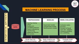
Feature scaling in machine learning is one of the most critical steps during the pre-processing of data before creating a machine learning model.
Scaling can make a difference between a weak machine learning model and a better one.
The most common techniques of feature scaling are Normalization and Standardization.


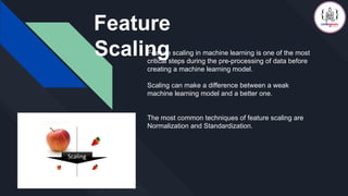
![Normalization is used when we want to bound our
values between two numbers, typically, between [0,1]
or [-1,1].
While Standardization transforms the data to have zero
mean and a variance of 1, they make our
data unitless.](https://image.slidesharecdn.com/machinelearning-4-260106075738-e8465623/85/Machine-Learning-basics-and-algorithm-pptx-11-320.jpg)


![[DSC Europe 25] Nikola Vasiljevic - Player segmentation by combat playstyles ...](https://cdn.slidesharecdn.com/ss_thumbnails/mnvbf0yvrwaqsipzrrv3-2-nikola-vasiljevic-player-segmentation-by-playstyles-in-action-shooter-games-260114111931-b4d766cd-thumbnail.jpg?width=640&height=640&fit=bounds)
![[DSC Europe 25] Slobodan Dolinic - Smart and Intelligent Green Region.pptx](https://cdn.slidesharecdn.com/ss_thumbnails/0bribinjsp6ghwtvsvor-2-sigre-slobodan-dolinic-260115093812-c9c10e90-thumbnail.jpg?width=640&height=640&fit=bounds)

![[DSC Europe 25] Ivan Lukovic & Marija Djukic - From Data to Value: Why Maturi...](https://cdn.slidesharecdn.com/ss_thumbnails/ahrfps8xr6knowwhacxh-1-ivan-marija-dsc-2025-ld-v1-presentation-260115093812-be21adfc-thumbnail.jpg?width=640&height=640&fit=bounds)


![[DSC Europe 25] Mijat Kustudic - Building Financial Intelligence with AI Agen...](https://cdn.slidesharecdn.com/ss_thumbnails/38y2lb5lse6wstegtvas-3-mijat-kustudic-building-financial-intelligence-with-ai-agents-260114111931-1a4783ce-thumbnail.jpg?width=640&height=640&fit=bounds)


![[DSC Europe 25] Elena Menshikova - AI-Powered Operational Excellence: Revolut...](https://cdn.slidesharecdn.com/ss_thumbnails/es6nholbqy3zaao2c2yd-2-elena-menshikova-data-ai-in-decision-making-260115093812-4fba8b38-thumbnail.jpg?width=640&height=640&fit=bounds)
![[DSC Europe 25] Danilo Djukanovic - From Vibes to KPIs: Turning Culture Into ...](https://cdn.slidesharecdn.com/ss_thumbnails/inqestws5wf0cik2glgv-3-danilo-djukanovic-from-vibes-to-kpis-presentation-260114111931-dacff81f-thumbnail.jpg?width=640&height=640&fit=bounds)

![[DSC Europe 25] Stefan Brankovic - #ResumeIsDead. AI-Powered Interviews and C...](https://cdn.slidesharecdn.com/ss_thumbnails/qnmbsv0xq3uysdrq3sev-2-stefan-brankovic-job-bolt-260114111931-a065aa3d-thumbnail.jpg?width=640&height=640&fit=bounds)


