(ANJALI) Dange Chowk Call Girls Just Call 7001035870 [ Cash on Delivery ] Pun...
M5.pdf
1. 3.1 Model of digital communication system
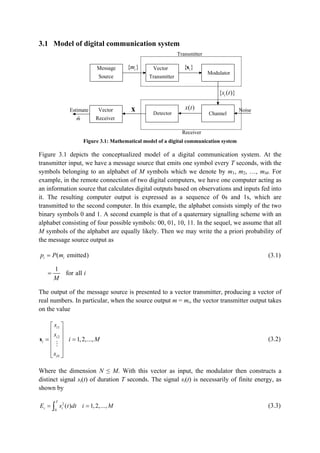
Figure 3.1: Mathematical model of a digital communication system
Figure 3.1 depicts the conceptualized model of a digital communication system. At the
transmitter input, we have a message source that emits one symbol every T seconds, with the
symbols belonging to an alphabet of M symbols which we denote by m1, m2, …, mM. For
example, in the remote connection of two digital computers, we have one computer acting as
an information source that calculates digital outputs based on observations and inputs fed into
it. The resulting computer output is expressed as a sequence of 0s and 1s, which are
transmitted to the second computer. In this example, the alphabet consists simply of the two
binary symbols 0 and 1. A second example is that of a quaternary signalling scheme with an
alphabet consisting of four possible symbols: 00, 01, 10, 11. In the sequel, we assume that all
M symbols of the alphabet are equally likely. Then we may write the a priori probability of
the message source output as
( emitted)
i i
p P m
(3.1)
1
for all i
M
The output of the message source is presented to a vector transmitter, producing a vector of
real numbers. In particular, when the source output m = mi, the vector transmitter output takes
on the value
1
2
1,2,...,
i
i
i
iN
s
s
i M
s
s
(3.2)
Where the dimension N ≤ M. With this vector as input, the modulator then constructs a
distinct signal si(t) of duration T seconds. The signal si(t) is necessarily of finite energy, as
shown by
2
0
( ) 1,2,...,
T
i i
E s t dt i M
(3.3)
Message
Source
Vector
Transmitter
Modulator
Channel
Detector
Vector
Receiver
Estimate
m̂
Noise
{ }
i
m { }
i
s
{ ( )}
i
s t
( )
x t
x
Transmitter
Receiver
2. Note that the signal si(t) is real–valued. One such signal is transmitted every T seconds. The
particular signal chosen for transmission depends in some fashion on the incoming message
and possibly on the signals transmitted in preceding time slots. Its characterization also
depends on the nature of the physical channel available for communication.
3.2 Mathematical models of communication channels
In the theory of digital communication systems, the communication channel is usually
represented by a mathematical model which reflects the most important characteristics of the
transmission medium. As channel is the interface between the transmitter and the receiver of
the communication system, this mathematical model helps to connect the transmitter and
receiver mathematically. We describe briefly three popular models that are frequently used to
characterise communication channel.
3.1.1 Additive noise channel
The AWGN channel is assumed to have two characteristics:
1. The channel is linear, with a bandwidth that is large enough to accommodate the
transmission of the modulator output si(t) distortion.
2. The transmitted signal si(t) is perturbed by an additive, zero mean, stationary, white,
Gaussian noise process, denoted by W(t). The reasons for this assumption are that it
makes calculations tractable, and also it is a reasonable description of the type of
receiver noise present in many communication systems.
We refer to such a channel as an additive white Gaussian noise (AWGN) channel.
Accordingly, we express the received random process, X(t), as
( ) ( ) ( ), 0 , 1,2,...,
i
X t s t W t t T i M
(3.4)
We may thus model the channel as in Figure 3.2, where the noise process W(t) is represented
by the sample function w(t), and the received random process X(t) is correspondingly
represented by the sample function x(t). From here on, we refer to x(t) as the received signal.
Figure 3.2: Model of additive white Gaussian noise channel
3.1.2 Linear filter channel
In some physical channels, such as wire-line telephone channels, filters are used to band limit
the signals and prevent interference among signals. In such cases, the channels are generally
characterised by linear filter channel model. This model is shown in Figure 3.3. In this model,
the channel output x(t) for a channel input si(t) and filter impulse response h(t) is given by
( ) ( ) ( ) ( )
i
x t s t h t w t
(3.5)
Transmitted
Signal ( )
i
s t
+
+ Received
Signal ( )
x t
White Gaussian
noise ( )
w t
3. Where represents convolution. In this model, the characteristics of the filter representing
the channel does not change with time. So the filter impulse response h(t) does not depend on
the elapsed time between observation and application of input.
Figure 3.3: Model of linear filter channel with AWGN
3.1.3 Linear time variant filter channel
Channels such as underwater acoustic channels, ionospheric radio channels, mobile cellular
radio channels are modelled as linear time variant filter channels. Here the signal travels
through various paths and arrives at the receiver at different times. The impulse response of
the channel varies with the elapsed time, hence differently arrived signals see different
channel characteristics. This leads to dispersion of the signal in time as well as in frequency
domain. However, linearity of the system is still preserved, so, the principle of superposition
can be applied to these differently travelling signals (multipath). The model is described
mathematically as
( ) ( ) ( , ) ( )
i
x t s t h t w t
(3.6)
Where the time variant channel impulse response h(τ, t) is the response of the channel at time
t due to an impulse applied at time t – τ. In many cases the time – variant impulse response is
modelled as
1
( , ) ( ) ( )
L
k k
k
h t a t
(3.7)
Where {ak(t)}represents the time variant attenuation factor for the kth
propagation path among
L multipath and {τk} are the corresponding time delays.
Figure 3.4: Model of linear time variant filter channel with AWGN
3.3 Gram–Schmidt Orthogonalization Procedure:
According to the model of Figure 3.1, the task of transforming an incoming message mi, i = 1,
2,…, M, into a modulated wave si(t) may be divided into separate discrete–time and
continuous–time operations. The justification for this separation lies in the Gram–Schmidt
orthogonal procedure, which permits the representation of any set of M energy signals,
Transmitted
Signal ( )
i
s t
+
+ Received Signal
( ) ( ) ( ) ( )
i
x t s t h t w t
White Gaussian
noise ( )
w t
Linear Filter
( )
h t
Channel
Transmitted
Signal ( )
i
s t
+
+ Received Signal
( ) ( ) ( , ) ( )
i
x t s t h t w t
White Gaussian
noise ( )
w t
Linear time variant
filter ( , )
h t
Channel
4. {si(t)}, as linear combination of N orthonormal basis functions, where N ≤ M. That is to say,
we may represent the given set of real–valued energy signals s1(t), s2(t),…, sM(t), each of
duration T seconds, in the form:
,
1
( ) ( ), 0 , 1,2,...,
N
i i j j
j
s t s t t T i M (3.8)
Where the coefficients of the expansion are defined by
,
0
( ) ( ) , 1,2,..., , 1,2,...,
T
i j i j
s s t t dt i M j N (3.9)
The real valued basis function ϕ1(t), ϕ2(t),…,ϕN(t) are orthonormal, by which we mean:
0
1
( ) ( )
0
T
i j
if i j
t t dt
if i j
(3.10)
The first condition of Eq. (3.10) states that each basis function is normalized to have unit
energy. The second condition states that the basis functions ϕ1(t), ϕ2(t),…,ϕN(t) are orthogonal
with respect to each other over the interval 0 ≤ t ≤ T.
Given that the set of coefficients {sij}, j = 1, 2,…, N, operating as input, we may use
the scheme shown in Figure 3.5 (a) to generate the signal si(t), i = 1, 2, …, M, which follows
directly from Eq. (3.8). It consists of a bank of N multipliers, with each multiplier supplied
with its own basis function, followed by a summer. This scheme may be viewed as
performing a similar role to that of second stage or modulator in the transmitter of Figure 3.1.
Conversely, given the set of signals si(t), i = 1, 2, …, M, operating as input, we may use the
scheme shown in Figure 3.5 (b) to calculate the set of coefficients{sij}, j = 1, 2,…, N, which
follows directly from Eq. (3.9). This second scheme consists of a bank of N product–
integrators or correlators with a common input, and with each one supplied with its own basis
function. Such a bank of correlators may be used as the first stage or detector in the receiver
of Figure 3.5.
(a) (b)
Figure 3.5: (a) Scheme for generating the signal si(t) (b) Scheme for generating the set of coefficients {si(t)}
1( )
i
s t
1( )
t
( )
i
s t
2 ( )
i
s t
2 ( )
t
( )
iN
s t
( )
N t
1( )
i
s t
1( )
t
( )
i
s t
2 ( )
i
s t
2 ( )
t
( )
iN
s t
( )
N t
0
T
dt
0
T
dt
0
T
dt
5. The Gram-Schmidt orthogonalization procedure requires two steps to prove as indicated next.
Stage I: First, we have to establish whether or not the given set of signals s1(t), s2(t),…, sM(t)
is linearly independent. If not, then (by definition) there exists a set of coefficients a1, a2,…,
aM, not all equal to zero, such that we may write:
1 1 2 2
( ) ( ) ... ( ) 0, 0
M M
a s t a s t a s t t T
(3.11)
Suppose, in particular, that aM ≠ 0. Then, we may express the corresponding signal sM(t) as:
1 2 1
1 2 1
( ) ( ) ( ) ... ( )
M
M M
M M M
a a a
s t s t s t s t
a a a
(3.12)
Which implies that sM(t) may be expressed in terms of the remaining (M – 1) signals.
Consider, next, the set of signals s1(t), s2(t),…, sM – 1(t). Either this set of signals is linearly
independent, or it is not. If not, then there exists a set of numbers b1, b2,…, bM – 1, not all
equal to zero, such that:
1 1 2 2 1 1
( ) ( ) ... ( ) 0, 0
M M
b s t b s t b s t t T
(3.13)
Suppose that bM – 1 ≠ 0. Then, we may express sM – 1(t) as a linear combination of remaining
M – 2 signals, as shown by
2
1 2
1 1 2 2
1 1 1
( ) ( ) ( ) ... ( )
M
M M
M M M
b
b b
s t s t s t s t
b b b
(3.14)
Now, testing the set of signals s1(t), s2(t),…, sM – 1(t) for linear independence, and countinuing
in this fashion, it is clear that we will eventually end up with a linearly independent subset of
the original set of signals. Let s1(t), s2(t),…, sN (t) denote this subset of linearly independent
signals, where N ≤ M. The important point to note is that each member of the original set of
signals s1(t), s2(t),…, sM(t) may be expressed as a linear combination of this subset of N
signals.
Stage II: Next we wish to show that it is possible to construct a set of N orthonormal basis
functions ϕ1(t), ϕ2(t),…, ϕN (t) from the linearly independent signals s1(t), s2(t),…, sN (t). As a
starting point, define the first basis function as:
1
1
1
( )
( )
s t
t
E
(3.15)
Where E1 is the energy of the signal s1(t). Then, clearly, we have
1 1 1 11 1
( ) ( ) ( )
s t E t s t
(3.16)
Where the coefficient 11 1
s E
and ϕ1(t) has unit energy, as required.
6. Next, using the signal s2(t), we define the coefficient s21 as
21 2 1
0
( ) ( )
T
s s t t dt
(3.17)
We may thus define a new intermediate function
2 2 21 1
( ) ( ) ( )
g t s t s t
(3.18)
Which is orthogonal to ϕ1(t) over the interval 0 ≤ t ≤ T. Now, we are ready to define the
second basis function as:
2
2
2
2
0
( )
( )
( )
T
g t
t
g t dt
(3.19)
Substituting Eq. (3.18) in Eq. (3.19), using Eq. (3.10), we get the desired result
2 21 1
2 2
2 21
( ) ( )
( )
s t s t
t
E s
(3.20)
Where E2 is the energy of the signal s2(t). Continuing in this fashion, we may define
1
1
( ) ( ) ( )
i
i i ij j
j
g t s t s t
(3.21)
Where the coefficient sij, j = 1, 2,…, i – 1, are themselves defined by
0
( ) ( )
T
ij i j
s s t t dt
(3.22)
Then it follows readily that the set of functions
2
0
( )
( ) , 1,2,...,
( )
i
i T
i
g t
t i N
g t dt
(3.23)
form an orthonormal set. Since we have shown that each one of the derived subset of linearly
independent signals s1(t), s2(t),…, sN (t) may be expressed as a linear combination of the
orthonormal basis functions ϕ1(t), ϕ2(t),…, ϕN (t), it follows that each one of the original set of
signals s1(t), s2(t),…, sM (t) may be expressed as a linear combination of this set of basis
functions, as described in Eq. (3.8).
Example 1.1: Consider the signals s1(t), s2(t), s3(t) and s4(t) shown in Figure 3.6. We wish to
use the Gram-Schmidt orthogonalization procedure to find an orthonormal basis for this set
of signals.
7. We observe immediately that s4(t) = s1(t) + s3(t), which means that this set of signals is not
linearly independent. Accordingly, we base the Gram-Schmidt orthogonalization procedure
on a subset consisting of signals s1(t), s2(t) and s3(t), which are linearly independent.
Figure 3.6: (a) Set of signals to be orthonormalized (b) The resulting set of orthonormal functions
Step I: We note energy of signal s1(t) is:
2
1 1
0
( )
T
E s t dt
/3
2
0
(1)
3
T T
dt
The first basis function ϕ1(t) is therefore (From Eq. 3.15):
1
1
1
( )
( )
s t
t
E
3/ , 0 / 3
0, elsewhere
T t T
Step II: From Eq. (3.17), we find that the coefficient s21 equals to:
21 2 1
0
( ) ( )
T
s s t t dt
/3
0
3
(1)
3
T T
dt
T
t
1( )
s t
0
1
3
T
t
2 ( )
s t
0
1
2
3
T
t
3( )
s t
0
1
3
T T
t
4 ( )
s t
0
1
T
( )
a
t
1( )
t
0
3/ T
3
T
t
2 ( )
t
0 2
3
T
t
3( )
t
0 2
3
T T
3
T
3/ T 3/ T
( )
b
8. The energy of signal s2(t) is
2
2 2
0
( )
T
E s t dt
2 /3
2
0
2
(1)
3
T T
dt
The second basis function ϕ2(t) is therefore (From Eq. (3.20)):
2 21 1
2 2
2 21
( ) ( )
( )
s t s t
t
E s
3/ , / 3 2 / 3
0, elsewhere
T T t T
Step III: From Eq. (3.22), we find that the coefficient s31 equals to:
31 3 1
0
( ) ( ) 0
T
s s t t dt
and the coefficient s32 equals to:
2 /3
32 3 2
/3
0
3
( ) ( ) (1)
3
T
T
T
T
s s t t dt dt
T
The pertinent value of the intermediate function gi(t), with i = 3, is therefore (From Eq.
(3.21))
3 3 31 1 32 2
( ) ( ) ( ) ( )
g t s t s t s t
1, 2 / 3
0, elsewhere
T t T
Finally, using Eq. (3.23), we find that the third basis function ϕ3(t) is
3
3
2
3
0
/ 3, 2 / 3
( )
( )
0, elsewhere
( )
T
T T t T
g t
t
g t dt
The resulting basis functions ϕ1(t), ϕ2(t) and ϕ3 (t) are shown in Figure 3.6 (b). It is clear that
these three basis functions ate orthonormal, and that any of the original signals s1(t), s2(t),
s3(t) and s4(t) may be expressed as a linear combination of them.
9.
10.
11. 3.4 Geometrical representation of signals
In Gram–Schmidt Orthogonalization procedure, it was shown that a convenient set of
orthonormal basis functions {ϕj(t)}, j = 1, 2,…, N, can be used to represent each signal in the
set {si(t)}, i = 1, 2,…, M according to Eq. (3.8) and Eq. (3.9). Similarly, each signal in the set
is completely determined by the vector of its coefficients as given in Eq. (3.2).
The vector si is called the signal vector. Furthermore, if we conceptually extend our
conventional notion of two and three dimensional Euclidean spaces to an N dimensional
Euclidean space, we may visualize the set of M points in an N dimensional Euclidean space,
with mutually perpendicular axes labelled ϕ1, ϕ2,…, ϕN. This N dimensional Euclidean space
is called the signal space.
The idea of visualizing a set of energy signals geometrically, as described above, is of
fundamental importance. For example Figure 1.8 illustrates the case of a two dimensional
signal space with three signals, that is, N = 2 and M = 3.
Figure 3.7: Geometrical representation of signals for the case when N = 2 and M = 3
In an N dimensional Euclidean space, we may define lengths of vectors and angles
between vectors. It is customary to denote the length or norm of a signal vector si by symbol
‖si‖. The squared length of any signal vector si is defined to be the inner product or dot
product of si with itself. In the familiar case of N = 2 or 3, we have
2 2
1
( , )
N
i i i ij
j
s
s s s (3.24)
Where the sij are the elements of si. For large values of N, length is defined in the same way,
and Eq. (3.11) remained valid.
The cosine of the angle between two vectors is defined as the inner product of the two
vectors divided by the product of their individual norms. That is, the csine of the angle
1
s
1
1
2
2 3
1
2
3
1
2
3
1
2
3
0
2
s
3
s
12. between the vectors si and sj equal to the ratio (si, sj)/‖si‖‖sj‖ . The two vectors si and sj are thus
orthogonal or perpendicular if their inner product (si, sj) is zero.
There is an interesting relationship between the energy content of a signal and its
representation as a vector. By definition, the energy of a signal si(t) of duration T seconds is
equal to
2
0
( )
T
i i
E s t dt
(3.25)
Therefore, substituting Eq. (3.8) in Eq. (3.12), we get
0
1 1
( ) ( )
N N
T
i ij j ik k
j k
E s t s t dt
(3.26)
Interchanging the order of summation and integration
0
1 1
( ) ( )
N N T
i ij ik j k
j k
E s s t t dt
(3.27)
But since ϕj(t) form an orthogonal set, then, in accordance with the two conditions of Eq.
(3.10), we find that Eq. (3.14) reduces simply to
2
1
N
i ij
j
E s
(3.28)
Thus Eq. (3.11) and Eq. (3.15) shows that the energy of a signal si(t) is equal to the squared
length of the signal vector si representing it. In case of pair of signals si(t) and sk(t),
represented by the signal vector si and sk, respectively, we may similarly show that
2 2
1
( )
N
i k ij kj
j
s s
s s
2
0
[ ( ) ( )]
T
i k
s t s t dt
(3.29)
Where ‖si – sk‖ is the Euclidean distance between the points represented by the signal vectors
si and sk.
13. Noise analysis of digital communication system:
Figure 3.14: Digital communication system with AWGN channel
Consider a digital communication system with AWGN channel.
( ) ( ) ( )
i
r t s t w t
The response of the channel r(t) for the input signal si(t) is passed through a receiving filter.
( ) ( ) ( ) ( ) ( ) ( ) ( ) ( ) ( ) ( )
i i
z t h t r t h t s t w t h t s t h t w t
0
( ) ( ) ( )
i
z t a t w t
The filter output z(t) is sampled at t = iTb. After sampling at t = Tb
0
( ) ( ) ( )
b i b b
z T a T w T
For simplicity the above equation can be written as:
0
i
z a w
Here, z, ai and w0 indicates some values but not function of time.
Case – 1: Assume that there is no signal at the input of the receiver
Therefore
z = w0,
where w0 is a sample of a random variable W0 with zero mean N0/2 variance. So, the
probability distribution function (PDF) of random variable ‘Z’ is:
2
0
0
1
( ) exp
Z
z
f z
N
N
The PDF of random variable ‘Z’ is shown in Figure 1.16
th
V
( )
i
S t Threshold
Comparator
Filter
( )
w t
( )
r t ( )
z t
b
t T
[ ]
b
z nT Decision
Output
Simply
z
14. Figure 1.16
Figure 1.17
Case – II: Assume that there binary symbol ‘1’ is present at input and let us consider ‘a1’ is
the data symbol corresponding to ‘1’. Therefore
z = a1 + w0,
Here ‘z’ is a sample of random variable Z with a1 mean N0/2 variance. So, PDF of random
variable ‘Z’ is:
2
1
0
0
1 ( )
( /1) exp
Z
z a
f z
N
N
The PDF of random variable ‘Z’ is shown in Figure 1.17
Figure 1.18
Case – III: Assume that there binary symbol ‘0’ is present at input and let us consider ‘a2’ is
the data symbol corresponding to ‘0’.
Therefore z = a2 + w0,
15. Here ‘z’ is a sample of random variable Z with a2 mean N0/2 variance.
So, PDF of random variable ‘Z’ is:
2
2
0
0
1 ( )
( / 0) exp
Z
z a
f z
N
N
The PDF of random variable ‘Z’ is shown in Figure 1.18
When binary ‘1’ is transmitted, then error occurs at z < 1 2
2
a a
with a probability
1 2
[1]
2
e
a a
P P z
Similarly, when binary ‘0’ is transmitted, then error occurs at z > 1 2
2
a a
with a probability
1 2
[0]
2
e
a a
P P z
So, probability of error for binary ‘1’ as shown in Figure 1.19 is:
1 2
2
[1] ( /1)
a a
e Z
P f z dz
So, probability of error for binary ‘0’ as shown in Figure 1.20 is:
1 2
2
[0] ( / 0)
e Z
a a
P f z dz
Figure 1.19
Figure 1.20
16. Example: Consider a binary digital communication system with ‘0’ and ‘1’ transmission.
When binary ‘0’ is transmitted, the voltage at the input of the comparator can have any value
between – 0.25 V to 0.25 V with equal probability. When binary ‘1’ is transmitted, the
voltage at the input of the comparator can have any value between 0 V to 1 V with equal
probability. If the threshold voltage of the comparator is 0.2 V, then determine the average
probability of error.
Solution:
PDF of ‘z’ when ‘0’ is transmitted PDF of ‘z’ when ‘1’ is transmitted
When ‘1’ is transmitted, the error occurs (‘0’ will be detected) with a probability, that is:
Pe = P[z < 0.2]
Therefore,
0.2 0.2
0
[1] ( /1) 1 0.2
e Z
P f z dz dz
When ‘0’ is transmitted, the error occurs (‘1’ will be detected) with a probability, that is:
Pe = P[z > 0.2]
Therefore,
0.25
0.2 0.2
[0] ( / 0) 2 0.1
e Z
P f z dz dz
Average probability of error:
[0] [1] 0.2 0.1
0.15
2 2
e e
avg
P P
P
( / 0)
Z
f z
z
0.25
0.25
2
0 0.2
[0]
e
P
( /1)
Z
f z
z
1
1
0 0.2
[1]
e
P