Download to read offline


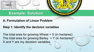
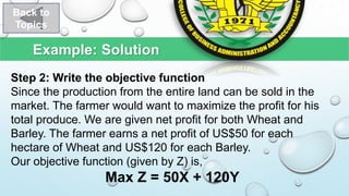


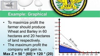


The document describes solving a linear programming problem through graphical representation and Excel Solver. It provides an example of a farmer who wants to maximize profits by deciding how many hectares to plant with wheat and barley, given costs, profits, land and labor constraints. The problem is formulated with decision variables for wheat and barley area, an objective function to maximize total profit, and constraints for budget, labor and total land area. The optimal solution is found to be planting wheat on 60 hectares and barley on 20 hectares, yielding maximum profit of $8,400.


![PENSHOPPE [autosaved]](https://cdn.slidesharecdn.com/ss_thumbnails/adv-141002033450-phpapp02-thumbnail.jpg?width=640&height=640&fit=bounds)


