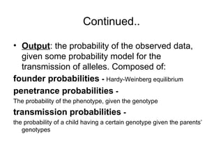
The document discusses genetic linkage analysis, a statistical method for associating genes with their chromosomal locations. It outlines key concepts like loci, alleles, and inheritance patterns including autosomal and X-linked traits, along with methodologies for conducting linkage mapping. Recent advancements such as the Superlink program are highlighted, which enhances computational efficiency in genetic analysis.

1. Genetic linkage analysis
Dotan Schreiber
According to a series of presentations by M. Fishelson

2. OutLine
• Introduction.
• Basic concepts and some background.
• Motivation for linkage analysis.
• Linkage analysis: main approaches.
• Latest developments.

3. “Genetic linkage analysis is a statistical
method that is used to associate
functionality of genes to their location on
chromosomes.“
http://bioinfo.cs.technion.ac.il/superlink/

4. The Main Idea/usage
:
Neighboring genes on the chromosome
have a tendency to stick together when
passed on to offsprings.
Therefore, if some disease is often passed
to offsprings along with specific marker-
genes , then it can be concluded that the
gene(s) which are responsible for the
disease are located close on the
chromosome to these markers.

5. Basic Concepts
• Locus
• Allele
• Genotype
• Phenotype

6. Dominant Vs. Recessive Allele
‫עיניים‬ ‫צבע‬ :‫קלאסית‬ ‫דוגמא‬
homozygote
heterozygote

7. (
se
)
X-Linked Allele
Most human cells contain 46 chromosomes:
• 2 sex chromosomes (X,Y):
XY – in males.
XX – in females.
• 22 pairs of chromosomes named autosomes.
Around 1000 human alleles are found only on the
X chromosome.

8. “…the Y chromosome essentially is reproduced via
cloning from one generation to the next. This
prevents mutant Y chromosome genes from being
eliminated from male genetic lines. Subsequently,
most of the human Y chromosome now contains
genetic junk rather than genes.”
http://anthro.palomar.edu/biobasis/bio_3b.htm

9. Medical Perspective
When studying rare disorders, 4 general patterns
of inheritance are observed:
• Autosomal recessive (e.g., cystic fibrosis).
– Appears in both male and female children of unaffected parents.
• Autosomal dominant (e.g., Huntington disease).
– Affected males and females appear in each generation of the
pedigree.
– Affected parent transmits the phenotype to both male and
female children.

10. Continued
..
• X-linked recessive (e.g., hemophilia).
– Many more males than females show the disorder.
– All daughters of an affected male are “carriers”.
– None of the sons of an affected male show the disorder or are
carriers.
• X-linked dominant.
– Affected males pass the disorder to all daughters but to none of
their sons.
– Affected heterozygous females married to unaffected males
pass the condition to half their sons and daughters.

11. Example
– After the disease is introduced into the family in generation #2, it
appears in every generation  dominant!
– Fathers do not transmit the phenotype to their sons 
X-linked!
1 2 3 4 5 6 7 8 9 10

12. Crossing Over
Sometimes in meiosis, homologous chromosomes exchange parts in
a process called crossing-over, or recombination.

13. Recombination Fraction
The probability  for a recombination
between two genes is a monotone, non-
linear function of the physical distance
between their loci on the chromosome.
Linkage)
No
(
5
.
0
)
ion
Recombinat
(
0
)
Linkage
( 

 P


14. Linkage
The further apart two genes on the same
chromosome are, the more it is likely that
a recombination between them will occur.
Two genes are called linked if the
recombination fraction between them is
small (<< 50% chance)

15. Linkage related Concepts
• Interference - A crossover in one region usually decreases
the probability of a crossover in an adjacent region.
• CentiMorgan (cM) - 1 cM is the distance between genes
for which the recombination frequency is 1%.
• Lod Score - a method to calculate linkage distances (to
determine the distance between genes).

16. Ultimate Goal: Linkage Mapping
With the following few minor problems:
– It’s impossible to make controlled crosses in
humans.
– Human progenies are rather small.
– The human genome is immense. The
distances between genes are large on
average.

17. Possible Solutions
• Make general assumptions:
Hardy-Weinberg Equilibrium – assumes certain probability
for a certain individual to have a certain genotype.
Linkage Equilibrium – assumes two alleles at different loci
are independent of each other.
• Incorporate those assumptions into
possible solutions:
Elston-Stewart method.
Lander-Green method.

18. Elston-Stewart method
• Input: A simple pedigree + phenotype
information about some of the people. These
people are called typed.
• Simple pedigree – no cycles, single pair of
founders.
founder
leaf
1/2

19. ..
Continued
• Output: the probability of the observed data,
given some probability model for the
transmission of alleles. Composed of:
founder probabilities - Hardy-Weinberg equilibrium
penetrance probabilities -
The probability of the phenotype, given the genotype
transmission probabilities -
the probability of a child having a certain genotype given the parents’
genotypes

20. ..
Continued
• Bottom-Up: sum conditioned probabilities
over all possible genotypes of the children
and only then on the possible genotypes
for the parents.
• Linear in the number of people.

21. Lander-Green method
• Computes the probability of marker
genotypes, given an inheritance vector.
P(Mi|Vi) at locus i
marker data at this
locus (evidence)
.
A certain inheritance
vector
.

22. Main Idea
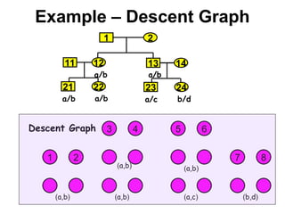
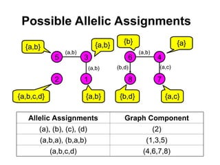
• Let a = (a1,…,a2f) be a vector of alleles assigned to
founders of the pedigree (f is the number of founders).
• We want a graph representation of the restrictions
imposed by the observed marker genotypes on the
vector a that can be assigned to the founder genes.
• The algorithm extracts only vectors a compatible with
the marker data.
• Pr[m|v] is obtained via a sum over all compatible vectors
a.

23. Example – marker data on a
pedigree
1 2
12
11
a/b
a/b
21
13
22
14
a/b
a/b
23 24
b/d
a/c

24. Example – Descent Graph
1 2
12
11
a/b
a/b
21
13
22
14
a/b
a/b
23 24
b/d
a/c
3 4 5 6
1 2 7 8
(
a,b
)
(
a,c
) (
b,d
)
(
a,b
)
(
a,b
)
(
a,b
)
Descent Graph

25. 3 4 5 6
1 2 7 8
(
a,b
)
(
a,c
) (
b,d
)
(
a,b
)
(
a,b
)
(
a,b
)
Descent Graph
1. Assume that paternally inherited genes are on the left.
2. Assume that non-founders are placed in increasing order.
3. A ‘1’ (‘0’) is used to denote a paternally (maternally)
originated gene.
 The gene flow above corresponds to the inheritance
vector: v = ( 1,1; 0,0; 1,1; 1,1; 1,1; 0,0 )

26. Example – Founder Graph
5 3
2 1
6 4
8 7
(
b,d
)
(
a,b
)
(
a,b
) (
a,c
)
(
a,b
)
Founder Graph
3 4 5 6
1 2 7 8
(
a,b
)
(
a,c
) (
b,d
)
(
a,b
)
(
a,b
)
(
a,b
)
Descent Graph

27. Find compatible allelic assignments
for non-singleton components
1. Identify the set of compatible alleles for each vertex.
This is the intersection of the genotypes.
5 3
2 1
6 4
8 7
(
b,d
)
(
a,b
)
(
a,b
) (
a,c
)
(
a,b
)
{a,b} ∩ {a,b} = {a,b} {a,b} ∩ {b,d} = {b}

28. Possible Allelic Assignments
5 3
2 1
6 4
8 7
(
b,d
)
(
a,b
)
(
a,b
) (
a,c
)
(
a,b
)
{
a,b
} {
a,b
}
{
a,b
} {
a,c
}
{
a
}
{
b
}
{
b,d
}
{
a,b,c,d
}
Graph Component
Allelic Assignments
(2)
(a), (b), (c), (d)
(1,3,5)
(a,b,a), (b,a,b)
(4,6,7,8)
(a,b,c,d)

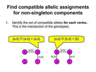
29. Computing P(m|v)
• If for some component there are no possible allelic
assignments, then P(m|v) = 0.
• The probability of singleton components is 1  we can
ignore them.
• Let ahi be an element of a vector of alleles assigned to the
vertices of component Ci.
]
Pr[
]
Pr[
}
:
{



i
C
j
j
j
hi a
a
]
Pr[
]
Pr[
}
:
{



i
hi A
a
h
hi
i a
C
]
Pr[
]
|
Pr[
1



m
i
i
C
v
m
over 2f elements
2
terms at most
Linear in the number of founders

30. Latest News: SuperLink
• Combines the covered approaches in one
unified program.
• Has other built-in abilities that increase its
computations efficiency.
• Claimed to be more capable and faster
than other related programs (by its own
makers).
• http://bioinfo.cs.technion.ac.il/superlink/

31. The
End