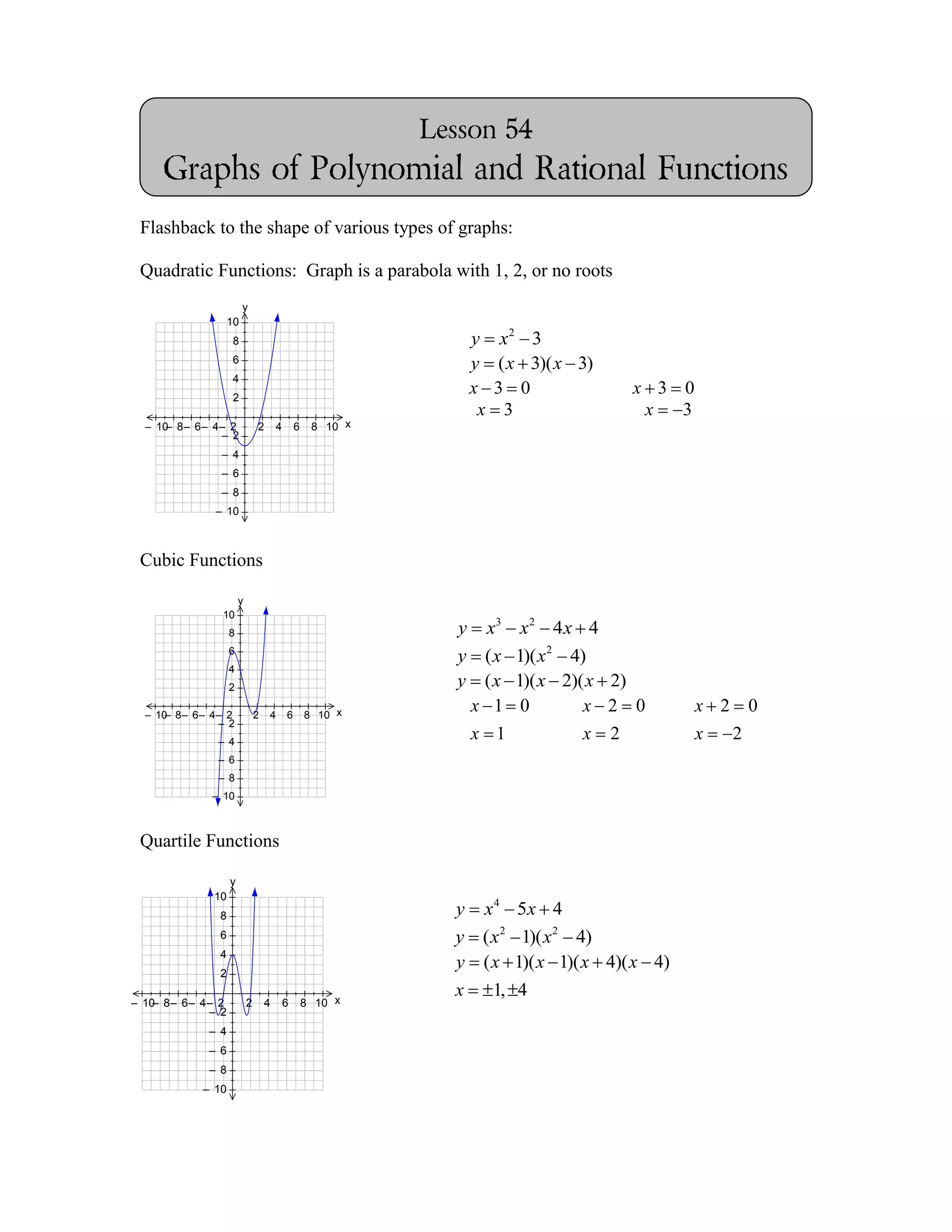
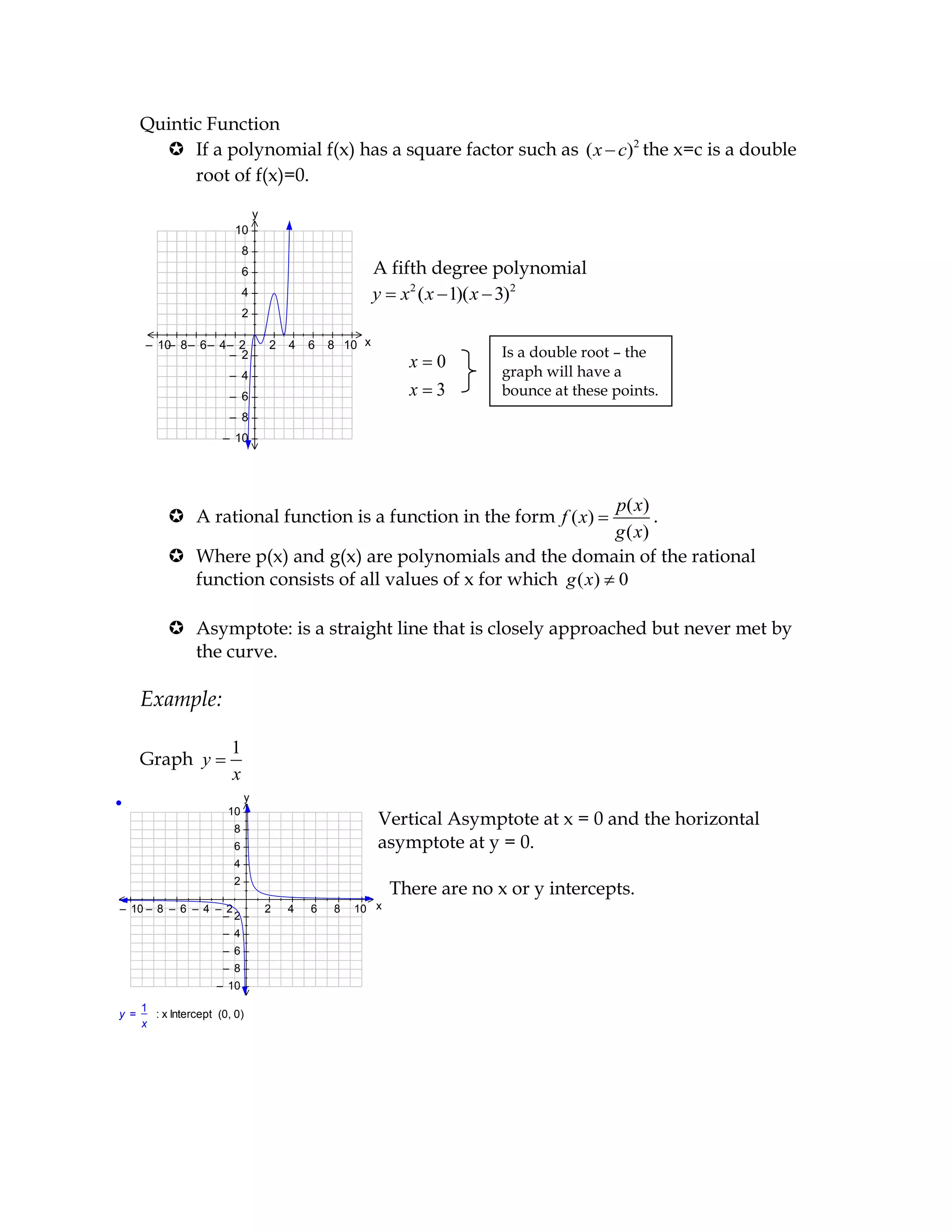
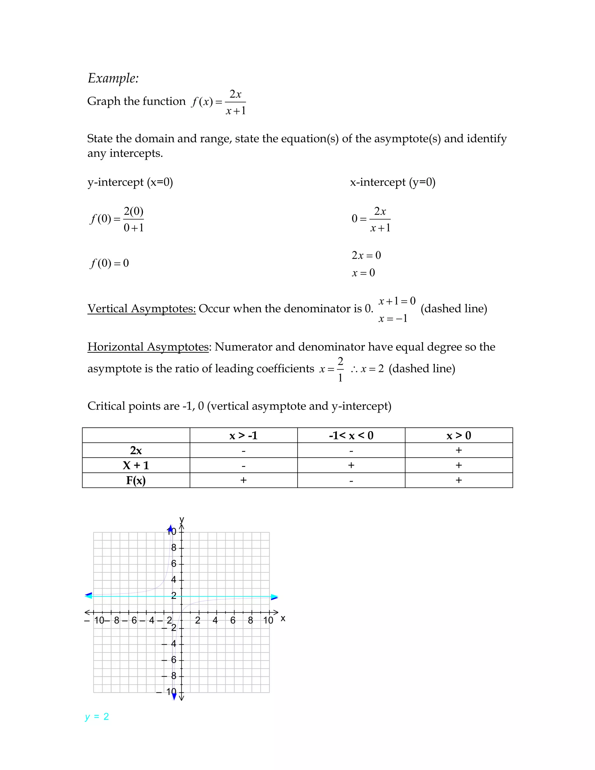
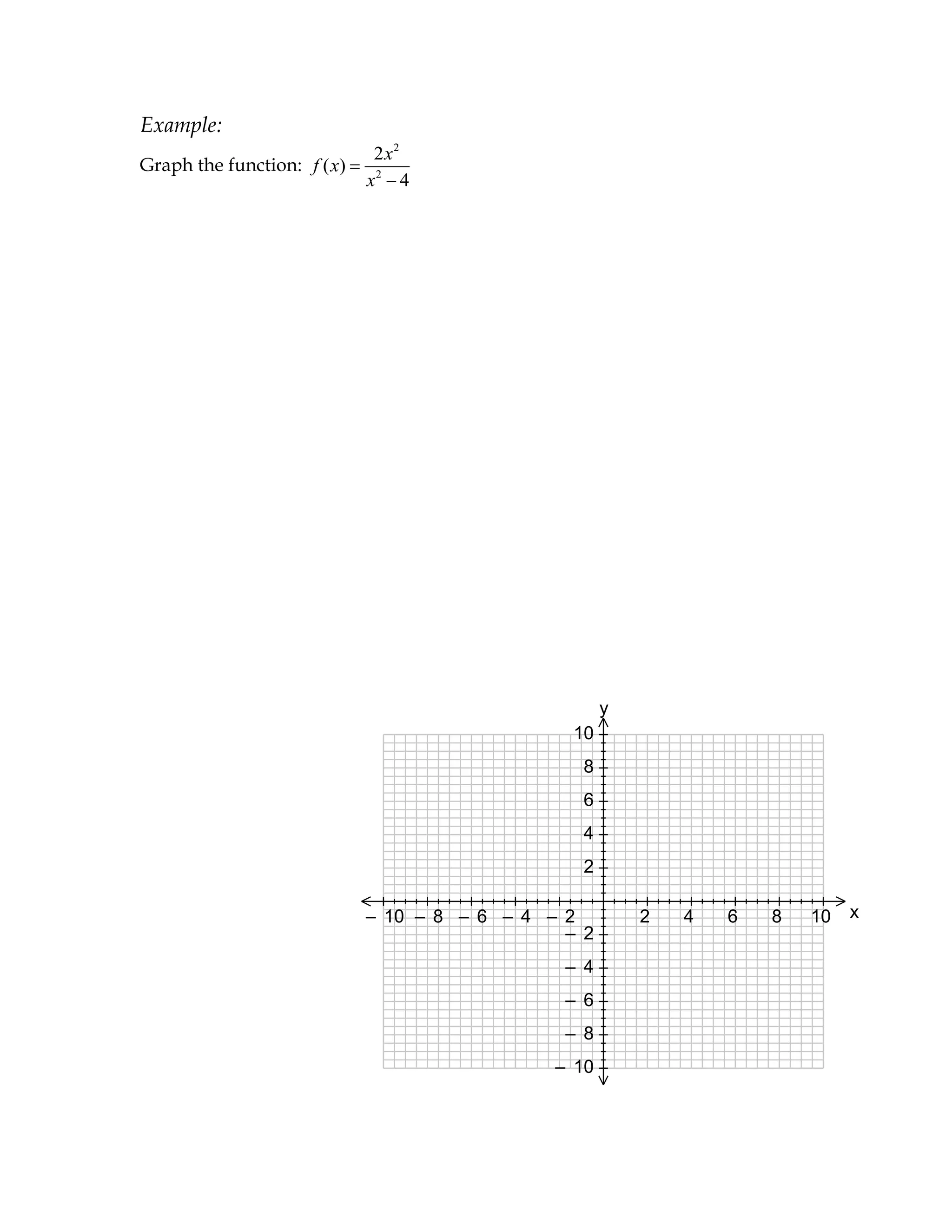
The document provides guidelines for graphing polynomial and rational functions. It discusses the key features of graphs of quadratic, cubic, quartic and quintic polynomials. It then discusses how to graph rational functions by identifying intercepts, asymptotes, discontinuities and using sign analysis to determine the positive and negative portions of the graph. An example rational function is graphed as an illustration.

1. Lesson 54
Graphs of Polynomial and Rational Functions
2– 2
10 10
8 8
6 6
4 4
2– 2
10 10
8 8
6 6
4 4
Flashback to the shape of various types of graphs:
Quadratic Functions: Graph is a parabola with 1, 2, or no roots
y
10
8 y x2 3
6 y ( x 3)( x 3)
4
2
x 3 0 x 3 0
x 3 x 3
– 10 8 – 6 – 4 – 2
– 2 4 6 8 10 x
– 2
– 4
– 6
– 8
2– 2
10 10
8 8
6 6
4 4
2– 2
10 10
8 8
6 6
4 4 – 10
Cubic Functions
y
10
8 y x3 x2 4x 4
6
y (x 1)( x2 4)
4
2 y (x 1)( x 2)( x 2)
– 10 8 – 6 – 4 – 2
– 2 4 6 8 10 x
x 1 0 x 2 0 x 2 0
– 2
– 4
x 1 x 2 x 2
– 6
2– 2
10 10
8 8
6 6
4 4 – 8
2– 2
10 10
8 8
6 6
4 4 – 10
Quartile Functions
y
10
8 y x 4 5x 4
6 y ( x2 1)( x2 4)
4
y ( x 1)( x 1)( x 4)( x 4)
2
x 1, 4
– 10 8 – 6 – 4 – 2
– 2 4 6 8 10 x
– 2
– 4
– 6
– 8
– 10

2. 2– 2
10 10
8 8
6 6
4 4
2– 2
10 10
8 8
6 6
4 4
Quintic Function
 If a polynomial f(x) has a square factor such as ( x c)2 the x=c is a double
root of f(x)=0.
y
10
8
6 A fifth degree polynomial
4 y x2 ( x 1)( x 3)2
2
– 10 8 – 6 – 4 – 2
– 2 4 6 8 10 x
– 2 Is a double root – the
x 0 graph will have a
– 4
– 6 x 3 bounce at these points.
– 8
– 10
p ( x)
 A rational function is a function in the form f ( x) .
g ( x)
 Where p(x) and g(x) are polynomials and the domain of the rational
function consists of all values of x for which g ( x) 0
 Asymptote: is a straight line that is closely approached but never met by
the curve.
Example:
1
2–=2
y
10 10
8 8
6 6
4 4
2– 2x
10 10
8 8
6 6
4 4
1
Graph y
x
y
10
8
Vertical Asymptote at x = 0 and the horizontal
6 asymptote at y = 0.
4
2
There are no x or y intercepts.
– 10 – 8 – 6 – 4 – 2 2 4 6 8 10 x
– 2
– 4
– 6
– 8
– 10
1
y = : x Intercept (0, 0)
x

3. Guidelines for Graphing Rational Functions:
1. Find and plot the y-intercept (if any) by evaluating f(0).
2. Find the zeros of the numerator (if any) by solving the equation p(x) = 0.
Then plot the corresponding intercepts.
3. Rational functions can be difficuly to graph by using only points.
Identifying discontinuities including asymptotes before you graph can
help you find key features so you can make a reasonable sketch of the
function.
4. Sketch the corresponding asymptotes by solving the equation of the
denominator q(x) = 0 to find the zeros of the denominator. The graph f(x)
has vertical asymptotes at each real zero of q(x).
5. Find and sketch the horizontal asymptote (if any) by using the following
rules:
a) If the degree of p(x) is less than the degree of g(x) then the line
y=0 is the horizontal asymptote.
a
b) If the degree of p(x) = the degree of g(x), then the line y is a
b
horizontal asymptote where a is the leading coefficient of p(x)
and b is the leading coefficient of g(x).
c) If the degree of p(x) is greater than the degree of the g(x), the
graph has no horizontal asymptote.
6. The graph of a rational function can be discontinuous at a value of x
without having an asymptote. This can occur if the numerator and the
denominator have a common factor.
7. Use sign analysis to show where the function portion is negative and
where it is positive.
8. Use smooth curves to complete the graph between and beyond the
vertical asymptotes.

4. Example:
2x
Graph the function f ( x)
x 1
State the domain and range, state the equation(s) of the asymptote(s) and identify
any intercepts.
y-intercept (x=0) x-intercept (y=0)
2(0) 2x
f (0) 0
0 1 x 1
2x 0
f (0) 0
x 0
x 1 0
Vertical Asymptotes: Occur when the denominator is 0. (dashed line)
x 1
Horizontal Asymptotes: Numerator and denominator have equal degree so the
2
asymptote is the ratio of leading coefficients x x 2 (dashed line)
1
Critical points are -1, 0 (vertical asymptote and y-intercept)
2–=22
y
10 10
8 8
6 6
4 4 x > -1 -1< x < 0 x>0
2– 2
10 10
8 8
6 6
4 4
2x - - +
X+1 - + +
F(x) + - +
y
10
8
6
4
2
– 10– 8 – 6 – 4 – 2 2 4 6 8 10 x
– 2
– 4
– 6
– 8
– 10
y = 2

5. Example:
2 x2
Graph the function: f ( x)
x2 4
2– 2
10 10
8 8
6 6
4 4
2– 2
10 10
8 8
6 6
4 4
y
10
8
6
4
2
– 10 – 8 – 6 – 4 – 2 2 4 6 8 10 x
– 2
– 4
– 6
– 8
– 10