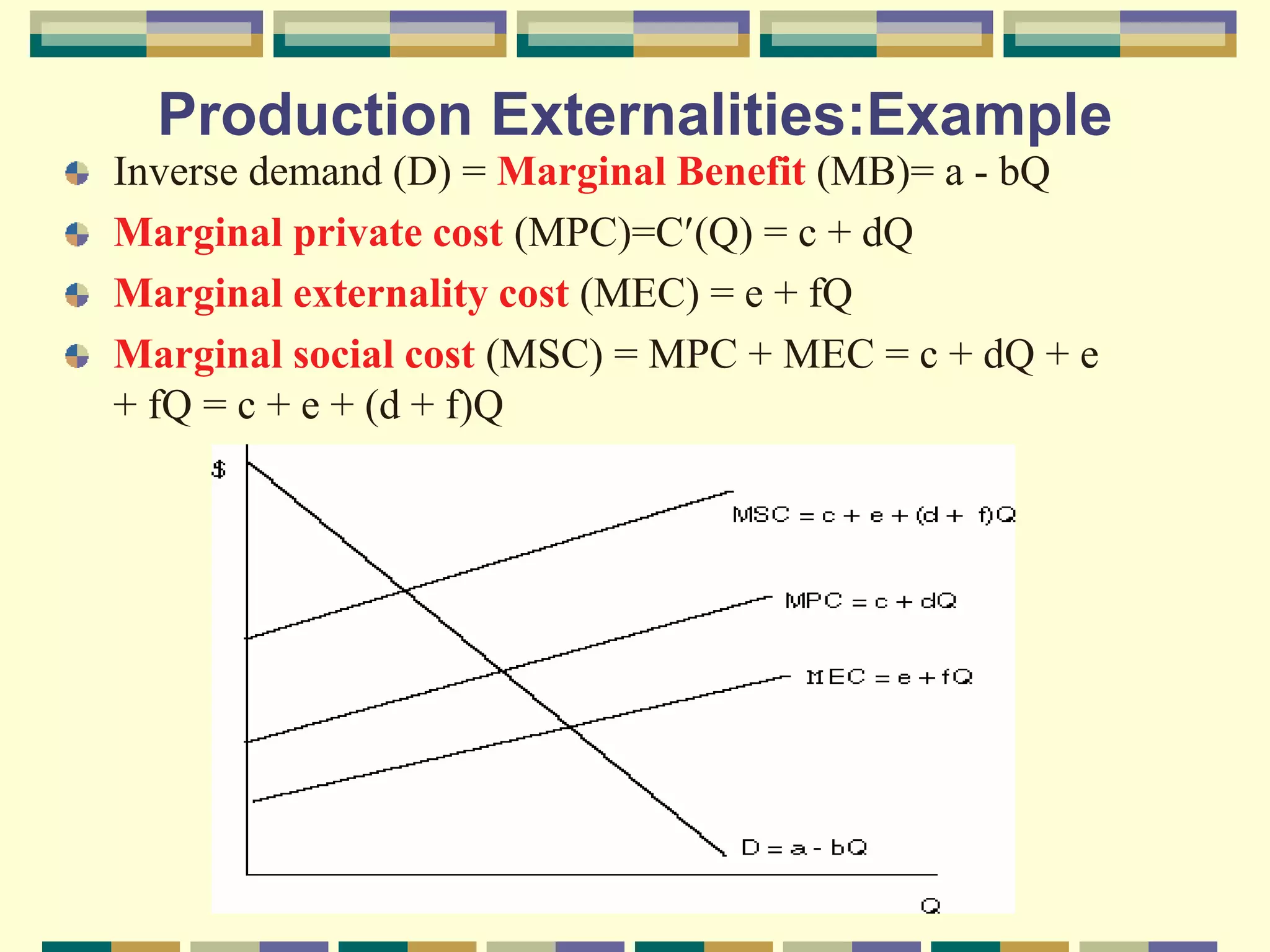
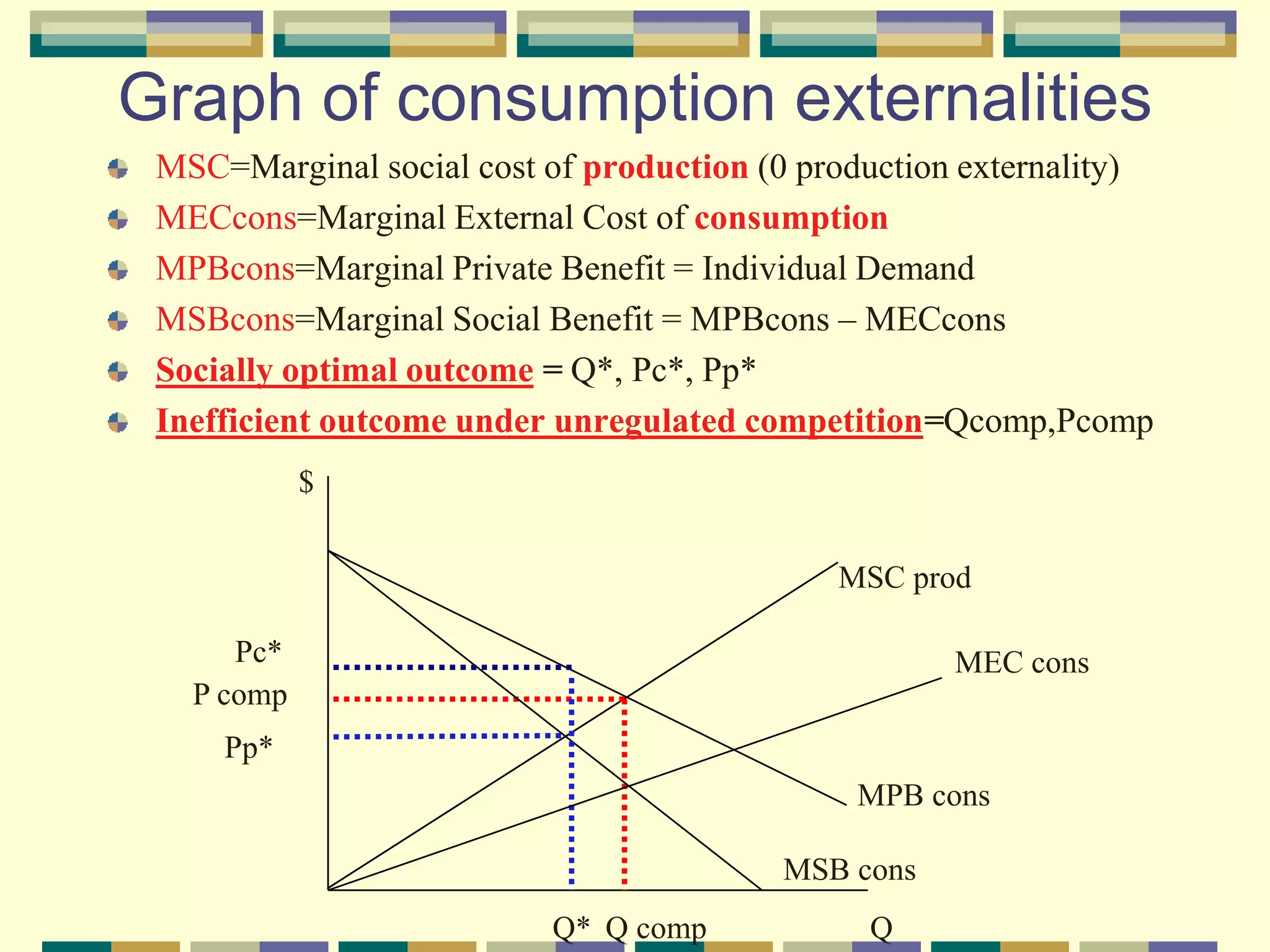
Chapter 4:
Negative Externalities
General Overview
Production Externalities
Policy 1: Externality Tax
Policy 2: Output-reduction Subsidy
Policy 3: Standards
Elasticity Effects on Magnitude of Externalities
Imperfect Competition and Externality Policy
Consumption Externalities
Externalities from Cigarette Smoking
The Economics of Illicit Drugs
General Overview
Externalities are a type of market failure
-prices in a market do not reflect the true marginal costs
and/or marginal benefits associated with the goods and
services traded in the market.
Externalities may be related to production
activities, consumption activities, or both.
-Production externalities: production activities of one
individual imposes costs/benefits on other individuals that
are not transmitted accurately through a market.
-Consumption externalities: consumption of an individual
imposes costs or benefits on other individuals that are not
accurately transmitted through a market.
Examples of production
externalities
 Air pollution from burning coal
 Ground water pollution from fertilizer use
 Food contamination and farm worker exposure to
toxic chemicals from pesticide use
 Irrigation water and consequential decline of
waterfowl population in nearby wildlife refuge
 Production of refrigerators using CFC’s
 Health issues resulting from gold mining
Production Externalities
$
A
MSC
MPC
MEC
D
B
P*
Q*
PC
QC
E
G
C
H
F
PP
Social optimum at B (where MSB=MSC)
Social Benefits = ABQ* O.
Social Costs = OBQ*.
Social Welfare = ABO.
Free market outcome at C
Social Benefits = ACQcO.
Social Costs = OCQc + OEC = OEQc.
Social Welfare = ABO - BEC.
Deadweight Loss = BEC.
Mathematical Representation of production externalities
The Social Welfare Maximization Problem is:
Max{W(Q)=B(Q)-C(Q)-E(Q)}
Q where:
Q = Output
B(Q) = Total Social Benefit of Producing Q.
C(Q) = Total Private Cost of Producing Q.
E(Q) = Total External Cost of Producing Q.
W(Q) =Social Welfare Function (Total Surplus From producing Q)
Social Welfare is maximized where Q satisfies the First-Order
Condition (FOC):
WQ=BQ (Q)-CQ (Q)-EQ (Q), which can be rearranged as
BQ(Q) = CQ(Q) + EQ(Q)
Where:
BQ(Q) =the partial derivative of B(Q) with respect to Q=MB
CQ(Q) = the partial derivative of C(Q) with respect to Q=MPC
EQ(Q) = the partial derivative of C(Q) with respect to Q=MEC
Socially optimum output, Q*, occurs when MB = MPC + MEC.
Unregulated competition with
externalities
Under unregulated competition, firms
maximize profits, resulting in the
FOC:BQ(Q) = CQ(Q), or MB = MPC.
When this FOC is solved for Q, call it QC,
we find that QC< Q* whenever MEC > 0.
Because QC Q*, QC is inefficient.
Policies to achieve social
optimum Q*
Three possible policies:
-Tax
-Subsidy
-Restriction, Standard, or Quota
Choice of policy affects the distribution of
economic benefits among producers, consumers
and government.
Targeting: Process of deciding which economic
variable to control to reduce externality.
Ex. Outputs, inputs, or the externality-generating
activity itself (i.e., the pollutant).
Policy 1: Tax-1
Externality Tax: t* = P* - PP=MEC (Q*), where
t* is the required market correction to achieve Q*
units of production.
Firms treat the tax rate as an additional component
of their marginal private cost; that is, a unit tax of
t* shifts the MPC curve upwards in a parallel
fashion by the distance t*.
$
A
MSC
MPC
MEC
D
B
P*
Q*
PC
QC
E
G
C
H
F
PP
Mathematical expression
t* = EQ(Q*) = MEC(Q*).
Private optimization problem:
Max {(Q)=PQ-C(Q)-t*Q}
Q
FOC:
Q(Q)-P-C Q(Q)-t*=0 or, P = CQ(Q) + t*.
Since P = MB at all points along the demand
curve, and t* = EQ(Q*), we can express the private
condition (which is identical to the condition for a
social optimum) under the tax as:
BQ(Q*) = CQ(Q*) + EQ(Q*)
Welfare implications of externality tax
Consumer surplus= ABP*
Producer surplus= OFPP
Government revenue= P*BFPP
$
A
MSC
MPC
MEC
D
B
P*
Q*
PC
QC
E
G
C
H
F
PP
Policy 1: Tax-2
Production tax: If the government knows
how much pollution is produced per unit of
production output, then it can set a tax on
production output that achieves the same
results as an externality tax. However, the
relationship between pollution and
production output is often very difficult to
estimate with any degree of precision.
Policy 1: Tax-3
Consumption Tax: Sales tax on polluting goods.
Demand curve for firms in the market shifts downward to
represent the net price of each unit sold. The net price, or
Net Marginal Benefit (NMB), is the Marginal Benefit of
consumers less the level of the sales tax (NMB = D - t*).
Q*=Social Optimum output
Pc*=Optimal Consumer price
Ps*=Pc*-t=net producer price
t=consumption tax
Policy 2: Output-reduction Subsidy
Subsidy = P* - PP for each unit of output that is
not produced.
If = the current level of output, firms in a
competitive industry have the following
objective: , and
FOC=
Optimal subsidy level: (i.e., the unit subsidy that
equates the optimal social and private outcomes)
S* = t* = MEC(Q*).
Q
 
Max PQ C Q Q Q S
Q
. ( ) ( )
    
Q P C Q S
   
' ( ) 0
Welfare implications of subsidy
Consumer surplus = ABP*.
Producer surplus = OFBP* + BGHF,where
BGHF = (P* - PP)·(Qc - Q*)].
Government expenditure = BGHF.
$
A
MSC
MPC
MEC
D
B
P*
Q*
PC
QC
E
G
C
H
F
PP
Problem with subsidy
In the long run, subsidies for pollution
reduction may actually increase pollution
because the subsidy may attract more firms
into the market.
Policy 3: Standards on
Pollution/Output
Command-and-control approach
through production quotas to restrict
output to Q*.
Welfare implications of quotas
Consumer surplus= ABP*
Producer surplus= OFBP* (larger than it is for
Externality Tax)
Government revenue= zero (smaller than it is for
Externality Tax) $
A
MSC
MPC
MEC
D
B
P*
Q*
PC
QC
E
G
C
H
F
PP
Quotas v. externality taxes
Producers prefer quotas to externality taxes
because they gain a larger share of social surplus.
If quota is transferable, producers will bid against
each other for the quota rights until the quota price
equals P*- PP.
-Whoever initially had the legal rights to the transferable
quota will earn quota rents equal to P*BFPP by selling
the quota rights.
-Buyer of the rights will be have surplus= PPFO.
*Note: producer surplus is the same as it is under an
externality tax. The quota rents is the same as
government revenue under the externality tax.
Elasticity Effects on the
Magnitude of Externalities
Pl
PE
MSC
MPC
D Inelastic
D elastic
Q
P
Ql
PC
QC
QE
PC, QC=Competitive price & quantity
PI, QI=Socially optimal price &
quantity, when D is inelastic
PE, QE=Socially optimal price &
quantity, when D is elastic
Elasticity and regulation
When demand is inelastic, the socially optimal
level of production, Qi, is not too far from the
competitive level of production, Qc. Therefore,
the inefficiency associated with a production
externality may be small, and it may not be worth
regulating the externality.
When demand is elastic, the socially optimal level
of production, Qe, is farther away from the
competitive level, Qc. In this case, the
inefficiency associated with the production
externality may be relatively large, and regulation
may be desirable.
Unexpected result of regulation?!
If demand is inelastic, pollution regulation
may increase producer profit.
-regulations that decrease production, such as a
quota, will move producers towards the monopoly
level of output. This decrease in turn will raise the
market price of the final product and increase
producers revenues.
The more inelastic the demand, the higher
the producer revenues under regulation!
Imperfect Competition and
Externality Policy
$
Q
D
MR
Qm Qc
Low MSC
Q*low
High MSC
Q*
High
MPC
A
B
Low MSC=small MEC
High MSC=large MEC
Unregulated competition=Qc
Monopoly=Qm
Low MSC
Optimal output, Q*low, is larger than the monopoly output, Qm.
In monopolistic market with low MSC, the optimal policy may be to
subsidize the polluting monopolist to produce more of the polluting
good.
$
Q
D
M
R
Qm Qc
Low MSC
Q*low
High
MSC
Q*
High
MPC
A
B
High MSC
Optimal output, Q*high, is smaller than the monopoly output, Qm.
In monopolistic market with high MSC, the optimal policy may be to
impose tax, T*=the distance AB. If this tax is imposed, MPC+t* will
intersect MR at Point B, which produces the optimal amount.
$
Q
D
M
R
Qm Qc
Low MSC
Q*low
High
MSC
Q*
High
MPC
A
B tax
Production Externalities:Example
Inverse demand (D) = Marginal Benefit (MB)= a - bQ
Marginal private cost (MPC)=C(Q) = c + dQ
Marginal externality cost (MEC) = e + fQ
Marginal social cost (MSC) = MPC + MEC = c + dQ + e
+ fQ = c + e + (d + f)Q
Social optimum
The Social Optimum is where MB = MSC
Marginal Benefit (MB)= a - bQ
Marginal social cost (MSC) = MPC + MEC = c + dQ
+ e + fQ = c + e + (d + f)Q
c  e  dQ  fQ  a  bQ Þ Q*
a  c  e
d  f  b
P* a  bQÞ P* a
ba bc be
d f b
 
 
 






Unregulated vs. Regulated Competition:
Unregulated competition: B Q(Q) = C Q(Q), MB = MPC
Marginal Benefit (MB)= a - bQ
Marginal Private Cost (MPC)=C(Q) = c + dQ
Regulated competition: B Q(Q*) = C Q(Q*) + t*
Impose tax t* = MEC(Q*) for regulated competition.
Marginal Externality Cost (MEC)= e + fQ
Q* at social optimal =
t* = MEC(Q*) = =
a  bQ  c  dQ Þ QC 
a  c
b  d
P  a  bQÞ PC  a 
ba bc
b  d
e f
a - c - e
d + f + b







e(d b) f(a c)
d f b
  
 
Q*
a  c  e
d  f  b
Unregulated Monopoly
Monopolist sets MPC=MR, where MR (marginal
revenue) is the derivative of R (total revenue), R= P(Q)Q
Demand = P(Q)= a – bQ
Marginal private cost (MPC)=C(Q) = c + dQ
  
Setting MPC = MR:
R aQ bQ
2
R abQ
( )Q MR  a  2bQ
c dQ a 2bQÞ QM 
a  c
d  2b
P  a bQ Þ PM a 
ba bc
d 2b






Unregulated Middleman
Unregulated middleman sets MR = MO, where MO
(marginal outlay) is the derivative of Outlay
MR=a-2bQ
Marginal private cost (MPC)=C(Q) = c + dQ
Outlay =MPC(Q)Q=(c + dQ)Q  MO = c + 2dQ
Setting MR = MO:
a-2bQ=c+dQ 
Price that middleman pays producers -substitute
QD into the equation for MPC:

Price that middleman charges consumers-
substitute QD into the equation for inverse demand:
QD 
a  c
2 b  d
( )
PP  c  dQ PP  c 
d
2
a  c
b d
PC  a  bQ  PC  a 
b
2
a  c
a  d
Consumption Externalities
We now turn to consumption externalities.
Consumption externality exists when one
individuals’ consumption imposes costs on
other individuals that are not transmitted
through a market.
Graph of consumption externalities
MSC=Marginal social cost of production (0 production externality)
MECcons=Marginal External Cost of consumption
MPBcons=Marginal Private Benefit = Individual Demand
MSBcons=Marginal Social Benefit = MPBcons – MECcons
Socially optimal outcome = Q*, Pc*, Pp*
Inefficient outcome under unregulated competition=Qcomp,Pcomp
P comp
Pp*
$
Q
MSC prod
MPB cons
Q comp
MSB cons
Q*
Pc* MEC cons
Externalities from Smoking
Health Costs Associated with Smoking:
 Smokers' health costs shared by society.
 Cost of family support (in case of early death).
 Risk to nonsmokers (second-hand smoke).
Estimated Death Toll (1989):
Estimated Annual external costs of smoking:
$ 35 billion (medical cost)
$ 20 billion (lost work)
$ 5 billion (fires, smoke, odor damage)
$ 60 billion (total cost)
Activity Annual deaths
Smoking 400,000
Drinking 150,000
Drugs 30,000
Policies to control cigarettes
(1) A cigarette tax or tobacco tax.
(2) A standard/quota to restrict quantities of
cigarettes and tobacco.
 Approximately 30 billion packs of
cigarettes are smoked annually.
 If marginal externality cost = average
externality cost, then the tax should be
$2.00 per pack ($60 billion of externality
cost / 30 billion packs).
Policy consequences
(1) Producers: Restriction on quantities may benefit
producers or distributors if elasticity of demand
is smaller than 1.
(2) Government: Tax revenues can be used to
compensate victims of smoking damages, or it
can be used in lieu of other distortionary taxes
(such as income taxes and sales taxes) to support
government programs.
(3) Unintended Consequences: May strengthen the
case for the legalization of drugs.
The Economics of Illicit Drugs
Should there be a drug legalization policy similar to the
one for cigarettes?
Proposals
 Legalize illicit drugs.
 Ban advertisement and sale to minors.
 Institute a tax on drugs.
Benefits:
 Increased government revenue.
 Reduced government costs (fewer prisoners and less drug
enforcement).
 Reduced crime.
Costs:
 Increased addiction.
 Legalization may induce more to try.
Economic impacts of drug policy
1. Legalization of drugs would shift income from the
illegal network of drug traffickers to government (taxes)
and legal marketers (pharmacies).
2. Drug producers may be better off if drug cartels
behave like the middlemen, since eliminating drug
trafficker middlemen may result in increased quantity
and higher producer prices.
3. Costs of crime enforcement may go down.
4. Consumer prices (inclusive of taxes) may go down
and quantity may go up. There may be higher health
costs associated with drug addiction.

lecture4 Negative externalities.pptx

  • 1.
    Chapter 4: Negative Externalities GeneralOverview Production Externalities Policy 1: Externality Tax Policy 2: Output-reduction Subsidy Policy 3: Standards Elasticity Effects on Magnitude of Externalities Imperfect Competition and Externality Policy Consumption Externalities Externalities from Cigarette Smoking The Economics of Illicit Drugs
  • 2.
    General Overview Externalities area type of market failure -prices in a market do not reflect the true marginal costs and/or marginal benefits associated with the goods and services traded in the market. Externalities may be related to production activities, consumption activities, or both. -Production externalities: production activities of one individual imposes costs/benefits on other individuals that are not transmitted accurately through a market. -Consumption externalities: consumption of an individual imposes costs or benefits on other individuals that are not accurately transmitted through a market.
  • 3.
    Examples of production externalities Air pollution from burning coal  Ground water pollution from fertilizer use  Food contamination and farm worker exposure to toxic chemicals from pesticide use  Irrigation water and consequential decline of waterfowl population in nearby wildlife refuge  Production of refrigerators using CFC’s  Health issues resulting from gold mining
  • 4.
    Production Externalities $ A MSC MPC MEC D B P* Q* PC QC E G C H F PP Social optimumat B (where MSB=MSC) Social Benefits = ABQ* O. Social Costs = OBQ*. Social Welfare = ABO. Free market outcome at C Social Benefits = ACQcO. Social Costs = OCQc + OEC = OEQc. Social Welfare = ABO - BEC. Deadweight Loss = BEC.
  • 5.
    Mathematical Representation ofproduction externalities The Social Welfare Maximization Problem is: Max{W(Q)=B(Q)-C(Q)-E(Q)} Q where: Q = Output B(Q) = Total Social Benefit of Producing Q. C(Q) = Total Private Cost of Producing Q. E(Q) = Total External Cost of Producing Q. W(Q) =Social Welfare Function (Total Surplus From producing Q) Social Welfare is maximized where Q satisfies the First-Order Condition (FOC): WQ=BQ (Q)-CQ (Q)-EQ (Q), which can be rearranged as BQ(Q) = CQ(Q) + EQ(Q) Where: BQ(Q) =the partial derivative of B(Q) with respect to Q=MB CQ(Q) = the partial derivative of C(Q) with respect to Q=MPC EQ(Q) = the partial derivative of C(Q) with respect to Q=MEC Socially optimum output, Q*, occurs when MB = MPC + MEC.
  • 6.
    Unregulated competition with externalities Underunregulated competition, firms maximize profits, resulting in the FOC:BQ(Q) = CQ(Q), or MB = MPC. When this FOC is solved for Q, call it QC, we find that QC< Q* whenever MEC > 0. Because QC Q*, QC is inefficient.
  • 7.
    Policies to achievesocial optimum Q* Three possible policies: -Tax -Subsidy -Restriction, Standard, or Quota Choice of policy affects the distribution of economic benefits among producers, consumers and government. Targeting: Process of deciding which economic variable to control to reduce externality. Ex. Outputs, inputs, or the externality-generating activity itself (i.e., the pollutant).
  • 8.
    Policy 1: Tax-1 ExternalityTax: t* = P* - PP=MEC (Q*), where t* is the required market correction to achieve Q* units of production. Firms treat the tax rate as an additional component of their marginal private cost; that is, a unit tax of t* shifts the MPC curve upwards in a parallel fashion by the distance t*. $ A MSC MPC MEC D B P* Q* PC QC E G C H F PP
  • 9.
    Mathematical expression t* =EQ(Q*) = MEC(Q*). Private optimization problem: Max {(Q)=PQ-C(Q)-t*Q} Q FOC: Q(Q)-P-C Q(Q)-t*=0 or, P = CQ(Q) + t*. Since P = MB at all points along the demand curve, and t* = EQ(Q*), we can express the private condition (which is identical to the condition for a social optimum) under the tax as: BQ(Q*) = CQ(Q*) + EQ(Q*)
  • 10.
    Welfare implications ofexternality tax Consumer surplus= ABP* Producer surplus= OFPP Government revenue= P*BFPP $ A MSC MPC MEC D B P* Q* PC QC E G C H F PP
  • 11.
    Policy 1: Tax-2 Productiontax: If the government knows how much pollution is produced per unit of production output, then it can set a tax on production output that achieves the same results as an externality tax. However, the relationship between pollution and production output is often very difficult to estimate with any degree of precision.
  • 12.
    Policy 1: Tax-3 ConsumptionTax: Sales tax on polluting goods. Demand curve for firms in the market shifts downward to represent the net price of each unit sold. The net price, or Net Marginal Benefit (NMB), is the Marginal Benefit of consumers less the level of the sales tax (NMB = D - t*). Q*=Social Optimum output Pc*=Optimal Consumer price Ps*=Pc*-t=net producer price t=consumption tax
  • 13.
    Policy 2: Output-reductionSubsidy Subsidy = P* - PP for each unit of output that is not produced. If = the current level of output, firms in a competitive industry have the following objective: , and FOC= Optimal subsidy level: (i.e., the unit subsidy that equates the optimal social and private outcomes) S* = t* = MEC(Q*). Q   Max PQ C Q Q Q S Q . ( ) ( )      Q P C Q S     ' ( ) 0
  • 14.
    Welfare implications ofsubsidy Consumer surplus = ABP*. Producer surplus = OFBP* + BGHF,where BGHF = (P* - PP)·(Qc - Q*)]. Government expenditure = BGHF. $ A MSC MPC MEC D B P* Q* PC QC E G C H F PP
  • 15.
    Problem with subsidy Inthe long run, subsidies for pollution reduction may actually increase pollution because the subsidy may attract more firms into the market.
  • 16.
    Policy 3: Standardson Pollution/Output Command-and-control approach through production quotas to restrict output to Q*.
  • 17.
    Welfare implications ofquotas Consumer surplus= ABP* Producer surplus= OFBP* (larger than it is for Externality Tax) Government revenue= zero (smaller than it is for Externality Tax) $ A MSC MPC MEC D B P* Q* PC QC E G C H F PP
  • 18.
    Quotas v. externalitytaxes Producers prefer quotas to externality taxes because they gain a larger share of social surplus. If quota is transferable, producers will bid against each other for the quota rights until the quota price equals P*- PP. -Whoever initially had the legal rights to the transferable quota will earn quota rents equal to P*BFPP by selling the quota rights. -Buyer of the rights will be have surplus= PPFO. *Note: producer surplus is the same as it is under an externality tax. The quota rents is the same as government revenue under the externality tax.
  • 19.
    Elasticity Effects onthe Magnitude of Externalities Pl PE MSC MPC D Inelastic D elastic Q P Ql PC QC QE PC, QC=Competitive price & quantity PI, QI=Socially optimal price & quantity, when D is inelastic PE, QE=Socially optimal price & quantity, when D is elastic
  • 20.
    Elasticity and regulation Whendemand is inelastic, the socially optimal level of production, Qi, is not too far from the competitive level of production, Qc. Therefore, the inefficiency associated with a production externality may be small, and it may not be worth regulating the externality. When demand is elastic, the socially optimal level of production, Qe, is farther away from the competitive level, Qc. In this case, the inefficiency associated with the production externality may be relatively large, and regulation may be desirable.
  • 21.
    Unexpected result ofregulation?! If demand is inelastic, pollution regulation may increase producer profit. -regulations that decrease production, such as a quota, will move producers towards the monopoly level of output. This decrease in turn will raise the market price of the final product and increase producers revenues. The more inelastic the demand, the higher the producer revenues under regulation!
  • 22.
    Imperfect Competition and ExternalityPolicy $ Q D MR Qm Qc Low MSC Q*low High MSC Q* High MPC A B Low MSC=small MEC High MSC=large MEC Unregulated competition=Qc Monopoly=Qm
  • 23.
    Low MSC Optimal output,Q*low, is larger than the monopoly output, Qm. In monopolistic market with low MSC, the optimal policy may be to subsidize the polluting monopolist to produce more of the polluting good. $ Q D M R Qm Qc Low MSC Q*low High MSC Q* High MPC A B
  • 24.
    High MSC Optimal output,Q*high, is smaller than the monopoly output, Qm. In monopolistic market with high MSC, the optimal policy may be to impose tax, T*=the distance AB. If this tax is imposed, MPC+t* will intersect MR at Point B, which produces the optimal amount. $ Q D M R Qm Qc Low MSC Q*low High MSC Q* High MPC A B tax
  • 25.
    Production Externalities:Example Inverse demand(D) = Marginal Benefit (MB)= a - bQ Marginal private cost (MPC)=C(Q) = c + dQ Marginal externality cost (MEC) = e + fQ Marginal social cost (MSC) = MPC + MEC = c + dQ + e + fQ = c + e + (d + f)Q
  • 26.
    Social optimum The SocialOptimum is where MB = MSC Marginal Benefit (MB)= a - bQ Marginal social cost (MSC) = MPC + MEC = c + dQ + e + fQ = c + e + (d + f)Q c  e  dQ  fQ  a  bQ Þ Q* a  c  e d  f  b P* a  bQÞ P* a ba bc be d f b            
  • 27.
    Unregulated vs. RegulatedCompetition: Unregulated competition: B Q(Q) = C Q(Q), MB = MPC Marginal Benefit (MB)= a - bQ Marginal Private Cost (MPC)=C(Q) = c + dQ Regulated competition: B Q(Q*) = C Q(Q*) + t* Impose tax t* = MEC(Q*) for regulated competition. Marginal Externality Cost (MEC)= e + fQ Q* at social optimal = t* = MEC(Q*) = = a  bQ  c  dQ Þ QC  a  c b  d P  a  bQÞ PC  a  ba bc b  d e f a - c - e d + f + b        e(d b) f(a c) d f b      Q* a  c  e d  f  b
  • 28.
    Unregulated Monopoly Monopolist setsMPC=MR, where MR (marginal revenue) is the derivative of R (total revenue), R= P(Q)Q Demand = P(Q)= a – bQ Marginal private cost (MPC)=C(Q) = c + dQ    Setting MPC = MR: R aQ bQ 2 R abQ ( )Q MR  a  2bQ c dQ a 2bQÞ QM  a  c d  2b P  a bQ Þ PM a  ba bc d 2b      
  • 29.
    Unregulated Middleman Unregulated middlemansets MR = MO, where MO (marginal outlay) is the derivative of Outlay MR=a-2bQ Marginal private cost (MPC)=C(Q) = c + dQ Outlay =MPC(Q)Q=(c + dQ)Q  MO = c + 2dQ Setting MR = MO: a-2bQ=c+dQ  Price that middleman pays producers -substitute QD into the equation for MPC:  Price that middleman charges consumers- substitute QD into the equation for inverse demand: QD  a  c 2 b  d ( ) PP  c  dQ PP  c  d 2 a  c b d PC  a  bQ  PC  a  b 2 a  c a  d
  • 30.
    Consumption Externalities We nowturn to consumption externalities. Consumption externality exists when one individuals’ consumption imposes costs on other individuals that are not transmitted through a market.
  • 31.
    Graph of consumptionexternalities MSC=Marginal social cost of production (0 production externality) MECcons=Marginal External Cost of consumption MPBcons=Marginal Private Benefit = Individual Demand MSBcons=Marginal Social Benefit = MPBcons – MECcons Socially optimal outcome = Q*, Pc*, Pp* Inefficient outcome under unregulated competition=Qcomp,Pcomp P comp Pp* $ Q MSC prod MPB cons Q comp MSB cons Q* Pc* MEC cons
  • 32.
    Externalities from Smoking HealthCosts Associated with Smoking:  Smokers' health costs shared by society.  Cost of family support (in case of early death).  Risk to nonsmokers (second-hand smoke). Estimated Death Toll (1989): Estimated Annual external costs of smoking: $ 35 billion (medical cost) $ 20 billion (lost work) $ 5 billion (fires, smoke, odor damage) $ 60 billion (total cost) Activity Annual deaths Smoking 400,000 Drinking 150,000 Drugs 30,000
  • 33.
    Policies to controlcigarettes (1) A cigarette tax or tobacco tax. (2) A standard/quota to restrict quantities of cigarettes and tobacco.  Approximately 30 billion packs of cigarettes are smoked annually.  If marginal externality cost = average externality cost, then the tax should be $2.00 per pack ($60 billion of externality cost / 30 billion packs).
  • 34.
    Policy consequences (1) Producers:Restriction on quantities may benefit producers or distributors if elasticity of demand is smaller than 1. (2) Government: Tax revenues can be used to compensate victims of smoking damages, or it can be used in lieu of other distortionary taxes (such as income taxes and sales taxes) to support government programs. (3) Unintended Consequences: May strengthen the case for the legalization of drugs.
  • 35.
    The Economics ofIllicit Drugs Should there be a drug legalization policy similar to the one for cigarettes? Proposals  Legalize illicit drugs.  Ban advertisement and sale to minors.  Institute a tax on drugs. Benefits:  Increased government revenue.  Reduced government costs (fewer prisoners and less drug enforcement).  Reduced crime. Costs:  Increased addiction.  Legalization may induce more to try.
  • 36.
    Economic impacts ofdrug policy 1. Legalization of drugs would shift income from the illegal network of drug traffickers to government (taxes) and legal marketers (pharmacies). 2. Drug producers may be better off if drug cartels behave like the middlemen, since eliminating drug trafficker middlemen may result in increased quantity and higher producer prices. 3. Costs of crime enforcement may go down. 4. Consumer prices (inclusive of taxes) may go down and quantity may go up. There may be higher health costs associated with drug addiction.