1. 1
Lecture 11, Slide 1EECS40, Fall 2003 Prof. King
Lecture #11
ANNOUNCEMENTS
• Homework Assignment #4 will be posted today
• Midterm #1: Monday Sept. 29th (11:10AM-12:00PM)
– closed book; one page (8.5”x11”) of notes & calculator allowed
– covers Chapters 1-5 in textbook (HW#1-4)
• Midterm Review Session: Friday 9/26 7-9PM, 277 Cory
• Extra office hours:
– Steve: 9/26 from 12-2PM
– Farhana: 9/27 from 1-3PM, 9/28 from 9-11AM
• Practice problems and old exam are posted online
OUTLINE
– Review: op amp circuit analysis
– The capacitor (Chapter 6.2 in text)
Lecture 11, Slide 2EECS40, Fall 2003 Prof. King
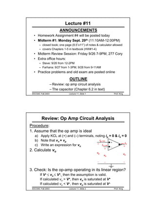
Review: Op Amp Circuit Analysis
Procedure:
1. Assume that the op amp is ideal
a) Apply KCL at (+) and (–) terminals, noting ip = 0 & in = 0
b) Note that vn = vp
c) Write an expression for vo
2. Calculate vo
3. Check: Is the op-amp operating in its linear region?
If V– ≤ vo ≤ V+,, then the assumption is valid.
If calculated vo > V+, then vo is saturated at V+
If calculated vo < V–, then vo is saturated at V–
+
–
+
vn
–
+
vp
–
ip
in
io
+
vo
–
+
–
+
vn
–
+
vp
–
ip
in
io
+
vo
–
2. 2
Lecture 11, Slide 3EECS40, Fall 2003 Prof. King
Op Amp Circuit Analysis Example
Consider the following circuit:
Assume the op amp is ideal.
a) Calculate vo if vs = 100 mV
b) What is the voltage gain vo/vs of this amplifier?
c) Specify the range of values of vs for which the
op amp operates in a linear mode
+
–
+
vo
–
–
+
vs
in
+
vp
–
+
vn
–
10 kΩ
1 kΩ 10 V
–10 V
Lecture 11, Slide 4EECS40, Fall 2003 Prof. King
Op Amp Circuit Analysis Example cont’d.
What if the op amp is not ideal?
Ri = 10 kΩ
Ro = 1 kΩ
A = 103
–
+
vs
10 kΩ
1 kΩ
+
vo
–
+
–
Ro
A(vp–vn)
Ri
+
vp
–
+
vn
–
3. 3
Lecture 11, Slide 5EECS40, Fall 2003 Prof. King
Re-draw the circuit
& analyze:
KCL @ node a:
KCL @ node b:
–
+
vs
1 kΩ
+
vn
–
+
–103(–vn)
1 kΩ
10 kΩ
10 kΩ
+
vo
–
1087.9 <≅−
s
o
v
v
a b
Lecture 11, Slide 6EECS40, Fall 2003 Prof. King
Effect of Load Resistance RL
KCL @ node b:
• For an ideal op amp (Ro = 0 Ω), vo does not depend on
the “load”. However, for a realistic op amp, it does.
–
+
vs
1 kΩ
+
vn
–
+
–103(–vn)
1 kΩ
10 kΩ
10 kΩ
+
vo
–
87.975.9 <≅−
s
o
v
v
a b
RL=1 kΩ
4. 4
Lecture 11, Slide 7EECS40, Fall 2003 Prof. King
The Capacitor
Two conductors (a,b) separated by an insulator:
difference in potential = Vab
=> equal & opposite charge Q on conductors
Q = CVab
where C is the capacitance of the structure,
positive (+) charge is on the conductor at higher potential
Parallel-plate capacitor:
• area of the plates = A
• separation between plates = d
• dielectric permittivity of insulator = ε
=> capacitance
d
A
C
ε
=
(stored charge in terms of voltage)
Lecture 11, Slide 8EECS40, Fall 2003 Prof. King
Symbol:
Units: Farads (Coulombs/Volt)
Current-Voltage relationship:
or
Note: vc must be a continuous function of time
+
vc
–
ic
dt
dC
v
dt
dv
C
dt
dQ
i c
c
c +==
C C
(typical range of values: 1 pF to 1 µF)
5. 5
Lecture 11, Slide 9EECS40, Fall 2003 Prof. King
Voltage in Terms of Current
)0()(
1)0(
)(
1
)(
)0()()(
00
0
c
t
c
t
cc
t
c
vdtti
CC
Q
dtti
C
tv
QdttitQ
+=+=
+=
∫∫
∫
Lecture 11, Slide 10EECS40, Fall 2003 Prof. King
You might think the energy stored on a capacitor is QV,
which has the dimension of Joules. But during charging,
the average voltage across the capacitor was only half the
final value of V.
Thus, energy is .2
2
1
2
1
CVQV =
Example: A 1 pF capacitance charged to 5 Volts
has ½(5V)2 (1pF) = 12.5 pJ
Stored Energy
6. 6
Lecture 11, Slide 11EECS40, Fall 2003 Prof. King
∫
=
=
=∫
=
=
∫
=
=
=⋅=
Final
Initial
c
Final
Initial
Final
Initial
ccc
Vv
Vv
dQvdt
tt
tt dt
dQVv
Vv
vdtivw
2CV
2
12CV
2
1Vv
Vv
dvCvw InitialFinal
Final
Initial
cc −∫
=
=
==
+
vc
–
ic
A more rigorous derivation
Lecture 11, Slide 12EECS40, Fall 2003 Prof. King
Integrating Amplifier
)0()(
1
)(
0
C
t
INo vdttv
RC
tv +−= ∫
+
–
vo
R in
+
vp
–
+
vn
–
ic
C
– vC +
vin