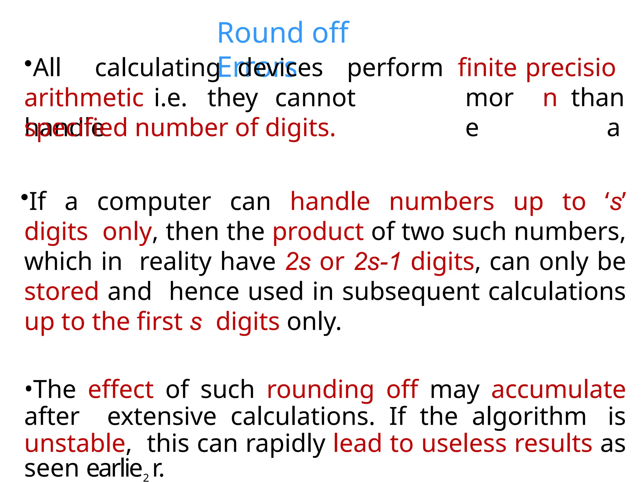
The document discusses error analysis in numerical calculations, focusing on round-off errors and truncation errors that can accumulate and lead to inaccurate results. It explains how the finite precision of computing devices can affect calculations and presents methods to reduce these errors, such as using higher-order polynomial approximations and Richardson's extrapolation. Additionally, it defines absolute and relative errors, as well as error bounds for operations like addition, subtraction, multiplication, and division.

1. Error
Analysis

2. Round off
Errors
arithmetic i.e. they cannot
handle
•All calculating devices perform finite
mor
e
precisio
n than
a
specified number of digits.
•If a computer can handle numbers up to ‘s’
digits only, then the product of two such numbers,
which in reality have 2s or 2s-1 digits, can only be
stored and hence used in subsequent calculations
up to the first s digits only.
•The effect of such rounding off may accumulate
after extensive calculations. If the algorithm is
unstable, this can rapidly lead to useless results as
seen earlie2 r.

3. Example of round-off error
We have already seen examples of round-
off errors when we tried to integrate
numerically
0
using the
recursion formula:
xn
1
yn   x  5
dx
n
3
n
y  5 y n1 
1

4. Example of round-off
error
4
3
2
y1  1  5 y0  .090
4 3
y 
1
 5 y  .165
3 2
y 
1
 5 y  .083
2 1
y 
1
 5 y  .050
1
4
0
dx
y0   x  5
 .182
•Round off errors lead to meaningless results
due to the instability of the algorithm.

5. 5
Truncation
Errors
•Truncation errors occur when a limiting process
is truncated before it has reached its limiting
value.
•A typical example may be a series which
converges after ‘n’ terms, is truncated i.e. cut-off
after the first
n/2 terms. The last n/2 terms represent in this
case the truncation error.
•Whenever a non-linear function is linearized, we
get a truncation error. The magnitude of the
truncation error is typically governed by the

6. Example of truncation
error
Nonlinear function of 𝑥, 𝑓𝑓(𝑥) is linearlized
about 𝑥:
𝑑
𝑥
0
𝑥0
0
𝑓𝑓(𝑥) = 𝑓𝑓(𝑥 ) +
𝑑
𝑓
𝑓
| (𝑥 − 𝑥
) + �q
u�a�d�r�a�t
i
c�
�t
e�r�m�s
𝑡𝑟𝑢𝑛𝑐𝑎𝑡𝑡𝑡𝑜𝑛
𝑒𝑟𝑟𝑜𝑟
To see a further example of truncation error
we consider numerical integration of the
definite integral:
𝑏
𝐼 = � 𝑦(𝑥) 𝑑𝑥
𝑎
6

7. 7
a series of trapezoids, each with a base width
Example of truncation
error
•Suppose we use the secant approximation to
evaluate the integral.
•The secant method, we recall, requires
approximating the non-linear function by straight
lines connecting successive function values.
•We assume that the ‘step size’ is constant i.e.
successive values of the independent variable x
e.g. xn and xn-1 differ by the constant step size ‘h’
•Thus the area between the curve y=f(x) and the
x

8. Trapezoidal
rule
•Hence this integration
scheme ‘trapezoidal rule’.
is called
the
y0
y1
2
y 3
y
y4
y5
h h
8
x
y=f(x)

9. Trapezoidal rule: truncation
error
•The ‘truncation error’, the error due to the
approximation of the nonlinear variation of y=f(x)
with a series of ‘linear variations’ is of the order h2
when h is small.
•Why is the error of the order h2 ?
2
9
2 2
5
4
4
 y )h
3
3
2
 y )h

1
( y  y )h 
1
( y
2

1
( y
2
0 1 1 2
I (h) 
1
( y  y )h 
1
( y  y )h

10. Reducing truncation
error
•This means that the error I - I(2h) for a step
size size of 2h is very nearly proportional to 4h2
while the
error I- I(h) for a step size of h
is very nearly proportional to h2.
•Hence
:
•Thus one can achieve arbitrarily high accuracy
by choosing a sufficiently small step size h.
•However reducing h means increased number of
function evaluations and higher computational
expense.
•Also for very small h, there may be an increase
in
I  I (h)

1
I  I (2h)
4
10
round off errors in the

11. Reducing truncation
error
•In order to avoid having to take very small step
sizes ‘h’, one can try approximating y(x) by a
higher order polynomial instead of a step wise
linear function.
•For instance the area under the curve y(x) may be
evaluated by approximating y(x) with piecewise
quadratic functions.
•The ‘truncation error’, would now be of the
order h3
rather than h2.
•Now
,
I  I (h)

1
I  I (2h) 8

12. Reducing truncation
error
•That would be an example of
polynomial
or ‘p’
refinement.
•Continuing with the secant (piece-wise
linear) approximation while reducing the size of the
step ‘h’
is an example of ‘h’ refinement.
•An alternative and highly efficient method for
reducing truncation error exists.
•It’s basic idea is due to Lewis Fry Richardson and
is known as ‘Richardson’s extrapolation’.
•For the current problem, it says that if we evaluate I
using the trapezoidal rule for several different

13. Richardson’s
Extrapolation
•By evaluating the integral for two step sizes h and 2h
and combining the results, we can come up with a
vastly improved solution.
•For example, for the secant approximation, we know:
I (h)  I  Kh2
and I (2h)  I  K 4h2
where K is a proportionality
constant
4(I (h)  I )  I (2h)  I
3I  4I (h)  I (2h)
to I(h) we can get a
much
better approximation to I with far lesser error
3
1
I (h)  I
(2h)
This leads to I  I (h) 
13
correction term
• Thus by adding a correction
term

14. Error
definitions
•Before entering into further details of error
analysis, it is appropriate to define a few terms
which we will need in our discussion.
•Let be a numerical approximation for a
quantity
.
a
~
whose exact value is a
a
14
•Then the absolute error is
a~  a
•The relative error is
a~ 
a~  a
if a  0

15. Error Bounds
•A bound on the magnitude of the error is
known as an error bound.
•Thus a bound on the absolute error is a
bound on:
a~  a
•A bound on the relative error is a bound on:
a~  a
a
15

16. 16
Error
Bounds
•The above error definitions hold in general for
vectors and matrices as well as scalars.
•However to hold for vectors and matrices we
have to define a proper magnitude (norm) for
the vector or matrix.
•The norm can then be used to define error
bounds for the vector or matrix.
•The error norm is a numerical value. When
dealing with numerical values we should be
clear about the distinction between the
number of decimals and number of digits in a
number.

17. 17
Decimals vs.
Digits
•The number of significant digits in a numerical
value does not include the zeros at the beginning
of the number, as these zeros only help denote
where the decimal point should be.
•However if counting the number of decimals,
one has to include the leading zeros to the
right of the decimal point.
•Example: .00548 has 3 significant digits but 5
decimals

18. Magnitude of
error
that the numerical approximation has 3
correct decimals.
•If the magnitudeof the error (whetherabsolute
or relative) in the numerical result does not
exceed
1
10t
2
then the numerical approximation, say, a~ ,
can be assured to have t correct decimals.
Example: If the absolute magnitude of error
does
2
18
not exceed say 1
103
or .0005 then we are
certain

19. Magnitude of
error
Example: Given a numerical solution .001234 and
an error magnitudeof .000004, we can
see that:
•Hence here t = 5 and the solution .001234 is
correct to 5 decimals.
which occupy
positions
where the unit is greater than or
equal to 2
1
10t
•The number of digits in
a~
(other than zeros at the beginning of the
number) are the number of significant digits
of a~ .
2
.000004 < .000005 =
1
105
.
19

20. Magnitude of
error
•The number of digits in .001234 which
occupy positions where the unit is greater than or
equal to
are the first 5
digits.
•However out of the first 5 digits, the first 2 digits
are zero. Hence the number of significant digits is
5-2 = 3
•We saw earlier that numerical solutions can be
severely affected by round off. However the “way”
round off is done can affect the severity of the
errors arising from it.
•If one simply “chops” off all decimals to the
right of the tth decimal place, then the round off
accumulate
2
1
105
20

21. Effects of
chopping
•This is because the errors consistentlyhave a
sign opposite to the true value.
•For instance, if the true solution a is known to
be
always positive, after round off by “chopping”,
the
operation
has no chance of cancelling out the
error from a
subsequent “chopping” operation.
•Similarly if the true solution a is known to be
always
negative, after round off by
“chopping”,
is
always positive, so again the errors from
repeated
round off operations keep
accumulating.
error a~  a is always negative.
•Thus, the error from one
“chopping”
a~  a
21

22. Effects of
chopping
•Depending on the number of significant digits, the
accumulation of round off errors may result in the
magnitude of cumulative error approaching the
true solution - yielding meaningless numerical
solutions.
•Roundoff errors due to chopping after t decimals
can lead to errors as large as 10-t .
•This can be seen, for instance, if .5559999….. is
chopped off after 3 decimals. In that case the
limiting value of the error is 1103
.
22

23. Rounding vs.
Chopping severe
man
y
•Thus ‘chopping’ has
alternative to
‘chopping’, ‘rounding’.
problems
.
computer
s
As
an
perfor
m
The rules for rounding are as follows. If the
magnitude then
:
by 1.
of the error does not exceed 1 2
10t
23
1.If the digit to the right of the tth decimal place is
less than1 2 10
,t
the tth decimal place is left
unchanged.
2.If the digit to the right of the tth decimal place
is greater than1 2 10t
, then the tth decimal place is

24. Rules for
Rounding
3.If the digit to the right of the tth decimal place is
exactly equal to 1 2 10t
, then the tth decimal place
is raised by 1 if it is odd, and left unchanged if it is
even.
•Since the probability of the tth decimal place being
odd or even is equal (each probability being equal
to half), if rule 3 is followed, the resulting error will
be positive or negative equally often.
•The errors will thus tend to cancel and not
accumulate.
•If the above rules are followed, then the error due

2
2
rounding off lies in the interval 

1
10t
,
1
10t

24

25. Superiority of
rounding
•This has to be compared to the fact that
‘chopping’ can lead to errors of magnitude as large
as 10-t
•The superiority of ‘rounding’ over ‘chopping’ is thus
clearly established.
•In addition, rounding errors have a greater
tendency to cancel each other out. This was
explicitly shown in case of rounding rule (3).
•However the combined effect of rules (1) and (2)
also favour cancellation of errors.
•This is because of two
reasons.
25

26. Superiority of
rounding
(a)The probability of the (t+1)th decimal being
greater is equal to the probability of the
(t+1)th
computation
than 1 2 10t
decimal being less than 1 2 10
.t
(b)The errors arising from application of rules (1)
and
(2) have the opposite sign.
•Irrespective of whether rounding or chopping is
used, for a numerical algorithm with a large
number of operations, round off errors due to
one computation are bound to propagate to
26

27. Bounds on
errors
•The subject of error propagation is complex.
However it is possible to come up with relatively
simple bounds on the error for basic operations
such as addition, subtraction, multiplication and
division.
•These bounds can allow estimation of errors for a
final numerical solution, if the error for each
intermediate step can be calculated.
which are
numerical
solutions for x1 andx2.
•Supposing that the bound on the absolute error in
x1 is
ε1 and the bound on the absolute error in x2 is
1
•Consider for instance
~x
2
and
~x
27

28. 28
Bounds on Addition &
Subtraction
Then we can write:
Hence the smallest possible value for
x1
x  ~x  
1 1
1
and the largest possible value for x1
x  ~x  
1
1
1
x  ~x

2 2
2
x  ~x
  ,
1 1 1

29. 29
Bounds on Addition &
Subtraction
Similarly the smallest possible value for x2
x2  ~x2
  2
while the largest possible value for x2
x2 
~x2   2
cannot be greater than the
largest
Since x1  x2
value of x1,minus the smallest value of x2, we
can write:
𝑥1 − 𝑥2 ≤ (𝑥�1 + 𝜀𝜀1) − (𝑥�2
− 𝜀𝜀2) (1)

30. 30
Bounds on Addition &
Subtraction
Similarly, since cannot be less than
the
x1  x2
smallest value of x1 ,minus the largest values of
x2, we can write:
(𝑥�1 − 𝜀𝜀1) − (𝑥�2 + 𝜀𝜀2) ≤ 𝑥1 − 𝑥2
(2)
Combining eqns. (1) and (2) we get:
(𝑥� 1 − 𝑥� 2) − (𝜀𝜀1 + 𝜀𝜀2) ≤ 𝑥1 − 𝑥2 ≤

31. Bounds on Addition &
Subtraction
Using a similar argument, it can be shown that:
(𝑥�1 + 𝑥�2) − (𝜀𝜀1 + 𝜀𝜀2) ≤ 𝑥1 + 𝑥2 ≤
(𝑥�1 + 𝑥�2) + (𝜀𝜀1 + 𝜀𝜀2)
(4)
Combining (3) and (4) we get:
2
31
1
(x  x )  (~x  ~x )  
 
1 2 1 2
2
1
(x  x )  (~x  ~x )  
 
1 2 1 2

32. 32
Bounds on Addition &
Subtraction
•We can write down the above result in terms of the
following theorem:
“The absolute error due to addition or subtraction of two
real numbers is bounded by the sum of the bounds on
the absolute error in each number”
•A similar bound can be obtained for multiplication
or division of two real numbers, but in this case the
bound involves relative rather than absolute error.

33. Bounds on Multiplication &
Division
Recall that the relative error r due to
approximation of the real number x by ~x
is defined as:
x
33
1
Suppose ~x
and
2
~
x
~x  x ~
r  , x  x(1 r)
are approximate
numerical and r1 and
r2 are the relative
solutions for x1 and
x2
errors in x1 and x2 .

34. Bounds on Multiplication &
Division
from
:
is found to
be:
Then we can write:
~x ~x  x (1 r )x (1 r )  x x (1 r )(1 r )
1 2 1 1 2 2 1 2 1 2
Thus the relative error in the product x1
x2 is:
(1 r1 )(1 r2 ) 1  r1  r2  r1r2  r1  r2, if r1  1,
r2  1
2 2
2
~
x
~
x x (1 r )
x (1 r )
1
 1 1
if r1  1, r2  1
1 r1
1 
r1  r2
1 r2 1 r2
 r1  r2
x2
Similarly the relative error in the
quotient x1
34

35. Bounds on Multiplication &
Division
Thus if 1 and 2 are bounds on the relative
errors r1 and r2 then it is clear that 1  2 is the
best upper bound for both 𝑟1 + 𝑟2 and 𝑟1 − 𝑟2
Thus we get the following theorem:
“In multiplication and division of real numbers,
the
bound on the relative error due to the operation is
equal to the sum of the bounds on the relative
errors in the operands”
35

36. Uses of error
analysis
•Error analysis enables the user make crucial
decisions that have an important bearing on the
accuracy and efficiency of the calculation.
•For instance if we consider the case where the
product x1x2 is to be calculated and x1 is known
up to 3 significant digits, and the true value of
x1 is of order one.
•We now need to calculate x2. From error
analysis it is clear that it does not make a lot of
sense to use
numerical methods to calculate x2 to
say
significant
6
36

37. Uses of error
analysis
in excess of since that may likely
worsen
the relative error in the product.
•The computational cost involved in the
numerical
calculation of x2 depends on the degree
of
accuracy with which we wish to calculate
x
•This is because we know that the relative error
in x1x2 may be as high as 1 2 103
(see slide 20)
•This follows from the fact that the bound on
the relative error in x1x2 is given by the sum on
the bounds on the relative errors in x1 and x2
•However it does make a lot of sense to
ensure that the relative error in the calculation
of x2 is not
1 2 103
37

38. Uses of error
analysis
•Hence knowledge of how the error
bounds
behave, enables us
to
improve the
efficiency
as
well as the accuracy of the numerical
analysis.
38

39. Error due to cancellation of
terms
•Numerical calculations involving subtractions
between two numbers, where the difference
between the operands is much less than any one
of the operands, are prone to large errors.
•Suppose we wish to calculate y  x1  x2 and the error
in the calculation of x1 and x2 are denoted by Δx1
and Δx2. Then the error in y, Δy is given as:
|∆𝑦| = |𝑥1 − 𝑥2| ≪ |∆𝑥1| + |∆𝑥2|
39
∴ |∆𝑦|
=
�
∆
𝑦
�
�|𝑦�|
�
�
�
�𝑦�
Since product
absolute
values is equal
to the absolute
value of the
|∆𝑥1| + |
∆𝑥2|
≪ |𝑥1 −
𝑥2|

40. General formula for error
propagation
•This general problem is of great interest
while performing experiments where empirical
data is fed
into mathematical
models.
40
Let us consider a function 𝑦 = (𝑥1, 𝑥2, 𝑥3 … . ,
𝑥𝑛 ) and suppose we want to estimate a bound for
the magnitude of the error in the value of the
function:
1
2
�
�
∆𝑦 = 𝑦(𝑥�1, 𝑥�2, … . , 𝑥�𝑛 ) −
𝑦(𝑥(0)
, 𝑥(0)
, … , 𝑥(0)
)
1
2
�
�
where 𝑥�1, 𝑥�2, … . , 𝑥�𝑛 are
the a
p
p
r
o
x
i
m
a
t
e values of
𝑥1, 𝑥2, … . , 𝑥𝑛 which have exact values
given by
𝑥
(0)
, 𝑥
(0)
, … , 𝑥
(0)

41. General formula for error
propagation
i
41
n
i
i
i

x
i
1
y
(~x)

x

y


 x
i
1
It can be shown that :
y 
y
(~x).x and
hence
∆𝑥𝑡
𝑡 = 𝑥� 𝑡
𝑡 − 𝑥(0)
∆𝑦 = 𝑦(𝐱
𝐱� ) −
𝑦(𝐱𝐱0)
𝑡
𝑡
n
Denotin
g:
1
2
�
�
𝐱
𝐱
� = (𝑥�1, 𝑥�2, … , 𝑥�𝑛 ) 𝐱𝐱0
= (𝑥(0)
, 𝑥(0)
. . , 𝑥(0)
)

42. 42
General formula for error
propagation
One can derive the above formula as follows:
Suppose we go from 𝗑0 to 𝐱
𝐱
� in 𝑛 steps,
changing one coordinate at a time. Thus for 𝑡
𝑡
= 1,2 … . , 𝑛 we set:
𝑡𝑡+1
𝑡𝑡+2
�
�
𝐱𝐱𝑡
𝑡 = (𝑥� 1 , 𝑥� 1 … 𝑥ˇ𝑡
𝑡 ,
𝑥(0)
, 𝑥(0)
, . . 𝑥(0)
)
Obviously,
𝐱𝐱𝑛 = 𝐱
𝐱
�

43. General formula for error
propagation
coordinate is changed
from
while the
rest
of the coordinates are left unchanged.
•Then by the mean value theorem, there
exists a
a such
that:
i i
x ~
to x
(0)
ξi xi1, xi

•In going from the (i 1)th
step to the ith
step, the
ith
43
𝑦(𝗑𝑡𝑡 ) − 𝑦(𝗑𝑡𝑡−1
=
𝜕
𝜕
𝑦
𝜕𝜕
𝑥𝑡
𝑡
) ( )
𝑡
𝑡
𝑡
𝑡
𝛏
𝛏. 𝑥
˜
�
− 𝑥
𝑡
�
�
(0
) �
�
�
𝑡𝑡+1
𝑡
𝑡
𝛏𝛏𝑡
𝑡 = 𝑥˜
� 1, … . 𝑥˜𝑡𝑡−1, 𝜉𝜉, 𝑥(0)
, …
𝑥(0)
� , 𝜉
𝜉 ∈ [𝑥(0)
, 𝑥˜𝑡
𝑡 ]
𝜕
𝜕
𝑥𝑡
𝑡
Hence one can write: 𝑦(𝗑𝑡𝑡 ) − 𝑦(𝗑𝑡𝑡−1) = 𝜕
𝜕
𝑦
(𝐱𝐱˜).
∆𝑥𝑡𝑡
(∗)
where the partial derivative of 𝑦 with respect to 𝑥𝑡
𝑡
at 𝛏𝛏𝑡
𝑡
is approximated by the partial derivative at the end
steps i.e.

44. i
n
i
i
n
i
i
n
i
i
i
i
i

i
1
y
(~x) 
x

i
1
y
(~x) 
x 
 y

 x
i
1
y
(~x) 
x
Hence y can be re - written as :
y 
x
i1 ) 
y
(~x)x
But from (*), y(x )  y(x
y


i1
i1
y(x )  y(x
)
General formula for error
propagation
Since y  y(xn )  y(x0 ), we can write :
n
44