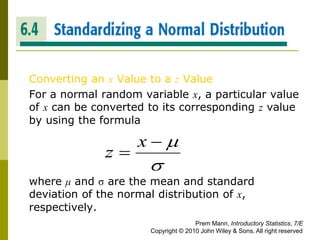
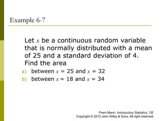
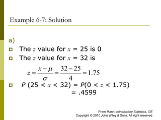
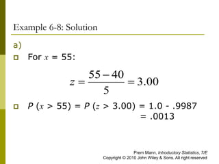
Lecture 14.ppt

Lecture 14
CHAPTER 6
CONTINUOUS RANDOM
VARIABLES AND THE
NORMAL
DISTRIBUTION
Prem Mann, Introductory Statistics, 7/E
Copyright © 2010 John Wiley & Sons. All right reserved

STANDARDIZING A NORMAL
DISTRIBUTION
Converting an x Value to a z Value
For a normal random variable x, a particular value
of x can be converted to its corresponding z value
by using the formula
where μ and σ are the mean and standard
deviation of the normal distribution of x,
respectively.




x
z

Example 6-6
Let x be a continuous random variable that
has a normal distribution with a mean of
50 and a standard deviation of 10. Convert
the following x values to z values and find
the probability to the left of these points.
a) x = 55
b) x = 35

Example 6-6: Solution
a) x = 55
P(x < 55) = P(z < .50) = .6915
50
.
10
50
55







x
z

Figure 6.31 z value for x = 55.

b) x = 35
P(x < 35) = P(z < -1.50) = .0668
35 50
1.50
10
x
z


 
   

Figure 6.32 z value for x = 35.

Example 6-7
Let x be a continuous random variable
that is normally distributed with a mean
of 25 and a standard deviation of 4.
Find the area
a) between x = 25 and x = 32
b) between x = 18 and x = 34

a)
 The z value for x = 25 is 0
 The z value for x = 32 is
 P (25 < x < 32) = P(0 < z < 1.75)
= .4599
75
.
1
4
25
32







x
z

Figure 6.33 Area between x = 25 and x = 32.

b)
 For x = 18:
 For x = 34:
 P (18 < x < 34) = P (-1.75 < z < 2.25 )
= .9878 - .0401 = .9477
75
.
1
4
25
18




z
25
.
2
4
25
34



z

Example 6-8
Let x be a normal random variable with
its mean equal to 40 and standard
deviation equal to 5. Find the following
probabilities for this normal distribution
a) P (x > 55)
b) P (x < 49)

a)
 For x = 55:
 P (x > 55) = P (z > 3.00) = 1.0 - .9987
= .0013
00
.
3
5
40
55



z

Figure 6.35 Finding P (x > 55).

b)
 For x = 49:
 P (x < 49) = P (z < 1.80) = .9641
80
.
1
5
40
49



z

Figure 6.36 Finding P (x < 49).

Example 6-9
Let x be a continuous random variable that
has a normal distribution with μ = 50 and σ
= 8. Find the probability P (30 ≤ x ≤ 39).

 For x = 30:
 For x = 39:
 P (30 ≤ x ≤ 39) = P (-2.50 ≤ z ≤ -1.38)
= .0838 - .0062 = .0776
50
.
2
8
50
30




z
38
.
1
8
50
39




z

Figure 6.37 Finding P (30 ≤ x ≤ 39).

Example 6-10
Let x be a continuous random variable
that has a normal distribution with a
mean of 80 and a standard deviation of
12. Find the area under the normal
distribution curve
a) from x = 70 to x = 135
b) to the left of 27

a)
 For x = 70:
 For x = 135:
 P (70 ≤ x ≤ 135) = P (-.83 ≤ z ≤ 4.58)
= 1 - .2033
= .7967 approximately
83
.
12
80
70




z
58
.
4
12
80
135



z

b)
 For x = 27:
 P (x < 27) = P (z < -4.42)
=.00 approximately
42
.
4
12
80
27




z

Figure 6.39 Area to the left of x = 27.

APPLICATIONS OF THE NORMAL
DISTRIBUTION
Section 6.2 through 6.4 discussed the
normal distribution, how to convert a
normal distribution to the standard normal
distribution, and how to find areas under a
normal distribution curve. This section
presents examples that illustrate the
applications of the normal distribution.

Example 6-11
According to a Sallie Mae and credit bureau
data, in 2008, college students carried an
average of $3173 debt on their credit cards
(USA TODAY, April 13, 2009). Suppose
that current credit card debts for all college
students have a normal distribution with a
mean of $3173 and a standard deviation of
$800. Find the probability that credit card
debt for a randomly selected college
student is between $2109 and $3605.

 For x = $2109:
 For x = $3605:
 P ($2109 < x < $3605)
= P (-1.33 < z < .54)
= .7054 - .0918
= .6136 = 61.36%
2109 3173
1.33
800
z

  
3605 3173
.54
800
z

 

Figure 6.40 Area between x = $2109 and x =
$3605.

Example 6-12
A racing car is one of the many toys
manufactured by Mack Corporation. The
assembly times for this toy follow a
normal distribution with a mean of 55
minutes and a standard deviation of 4
minutes. The company closes at 5 p.m.
every day. If one worker starts to
assemble a racing car at 4 p.m., what is
the probability that she will finish this job
before the company closes for the day?

 For x = 60:
 P(x ≤ 60) = P(z ≤ 1.25) = .8944
 Thus, the probability is .8944 that this
worker will finish assembling this racing
car before the company closes for the day.
60 55
1.25
4
z

  

Example 6-13
Hupper Corporation produces many types of soft
drinks, including Orange Cola. The filling machines
are adjusted to pour 12 ounces of soda into each
12-ounce can of Orange Cola. However, the actual
amount of soda poured into each can is not exactly
12 ounces; it varies from can to can. It has been
observed that the net amount of soda in such a
can has a normal distribution with a mean of 12
ounces and a standard deviation of .015 ounce.

Example 6-13
a) What is the probability that a randomly
selected can of Orange Cola contains 11.97 to
11.99 ounces of soda?
b) What percentage of the Orange Cola cans
contain 12.02 to 12.07 ounces of soda?

a)
 For x = 11.97:
 For x = 11.99:
 P (11.97 ≤ x ≤ 11.99)
= P (-2.00 ≤ z ≤ -.67) = .2514 - .0228
= .2286
00
.
2
015
.
12
97
.
11




z
67
.
015
.
12
99
.
11




z

Figure 6.42 Area between x = 11.97 and x = 11.99.

b)
 For x = 12.02:
 For x = 12.07:
 P (12.02 ≤ x ≤ 12.07)
= P (1.33 ≤ z ≤ 4.67) = 1 - .9082
= .0918
33
.
1
015
.
12
02
.
12



z
67
.
4
015
.
12
07
.
12



z

Figure 6.43 Area from x = 12.02 to x = 12.07.

Example 6-14
The life span of a calculator manufactured by
Texas Instruments has a normal distribution with a
mean of 54 months and a standard deviation of 8
months. The company guarantees that any
calculator that starts malfunctioning within 36
months of the purchase will be replaced by a new
one. About what percentage of calculators made
by this company are expected to be replaced?

 For x = 36:
 P(x < 36) = P (z < -2.25)
= .0122
 Hence, 1.22% of the calculators are
expected to be replaced.
25
.
2
8
54
36




z

Lecture 14.ppt

More Related Content

Similar to Lecture 14.ppt

Recently uploaded

Lecture 14.ppt