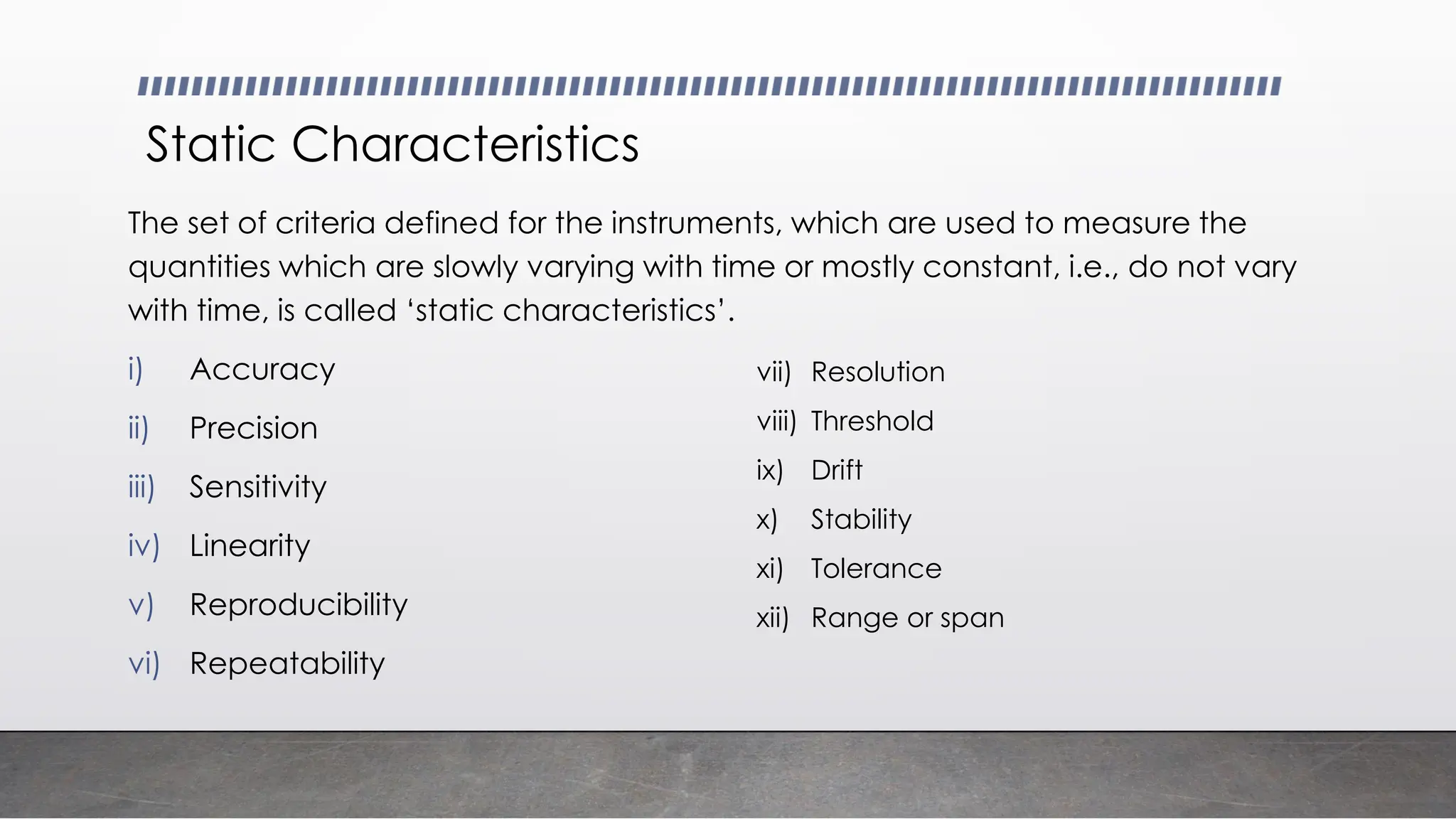
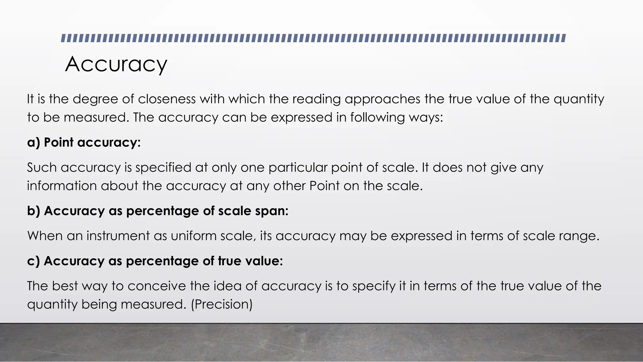
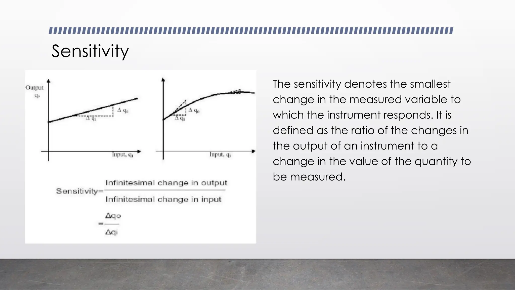
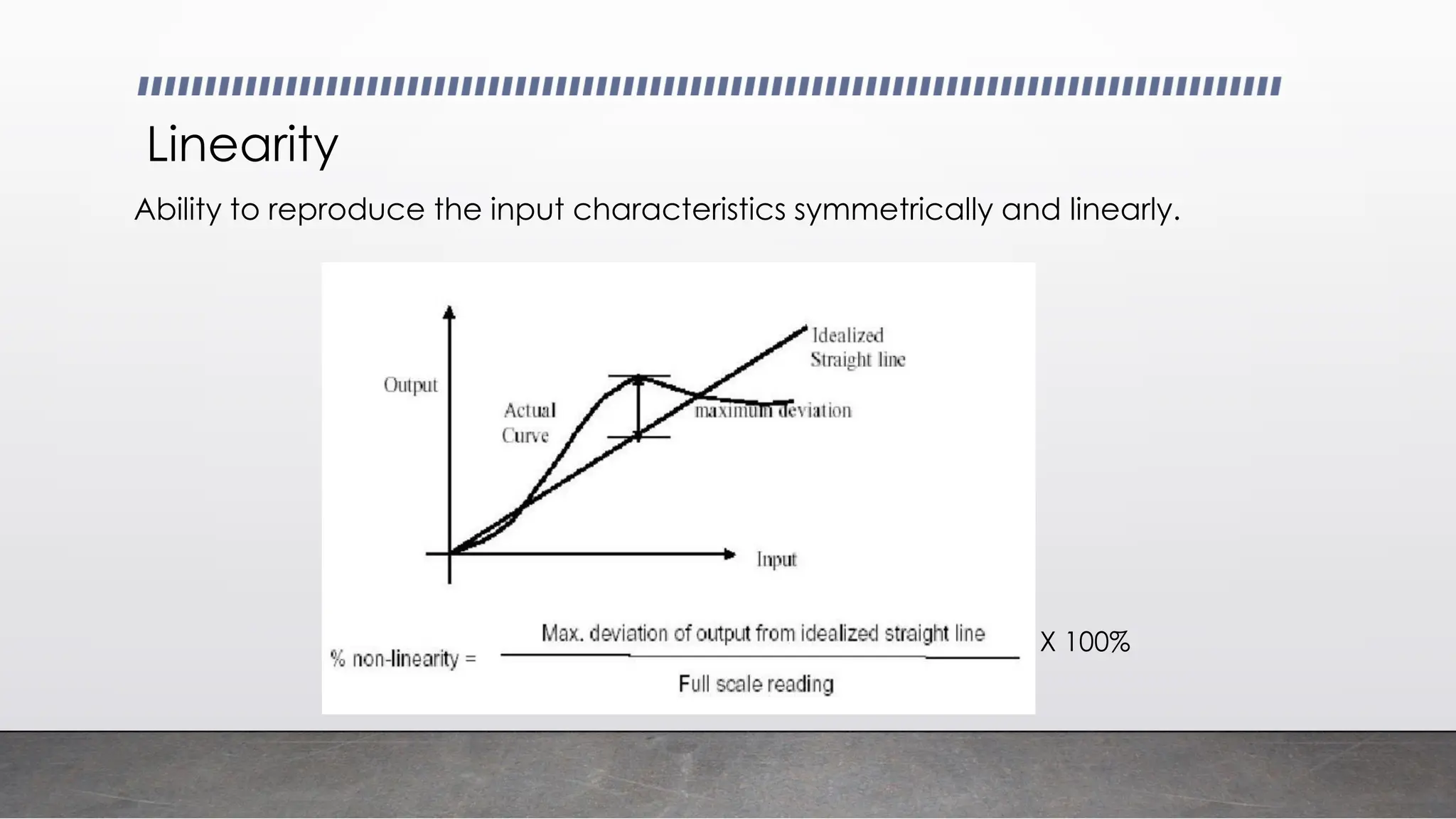
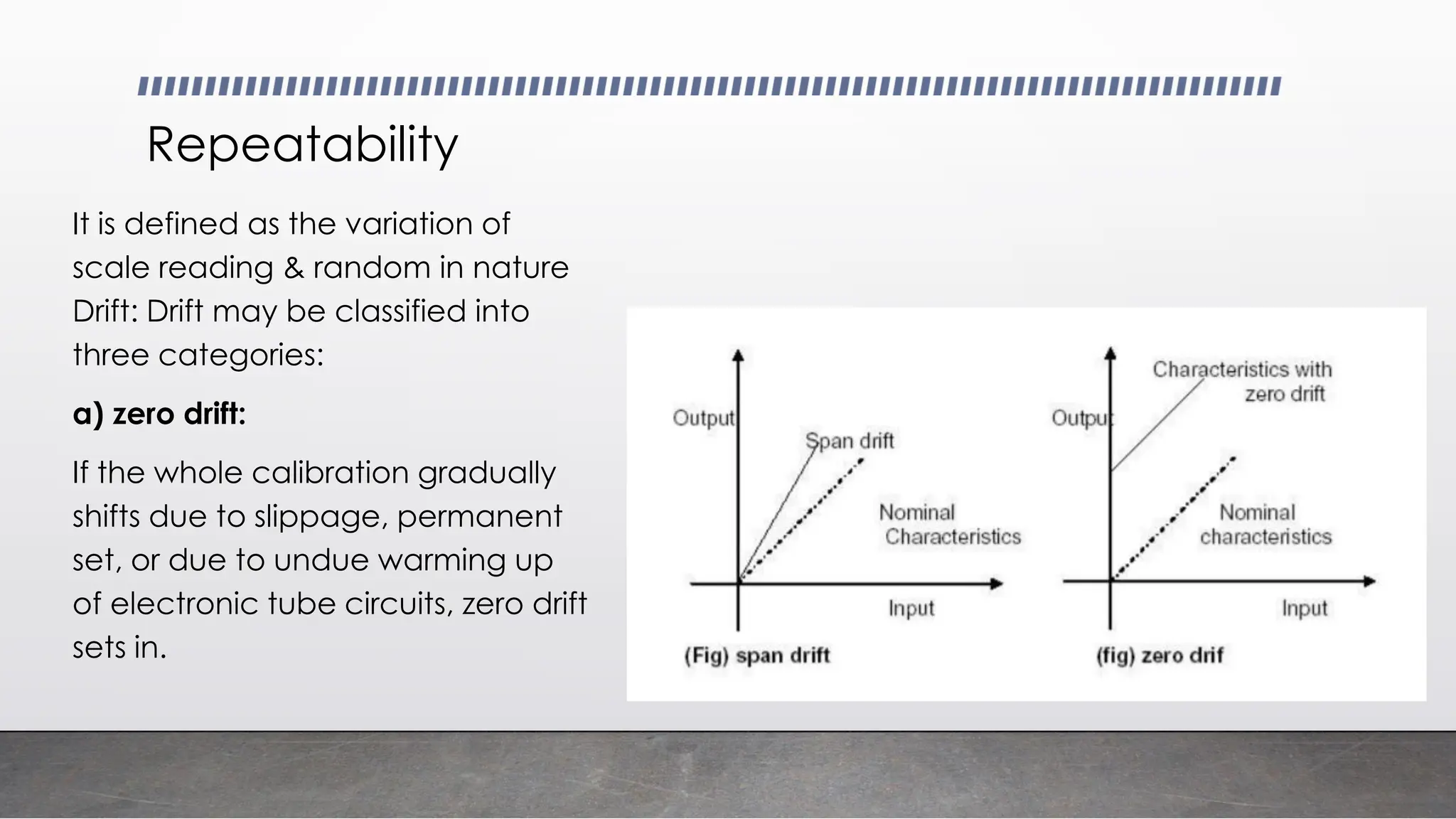
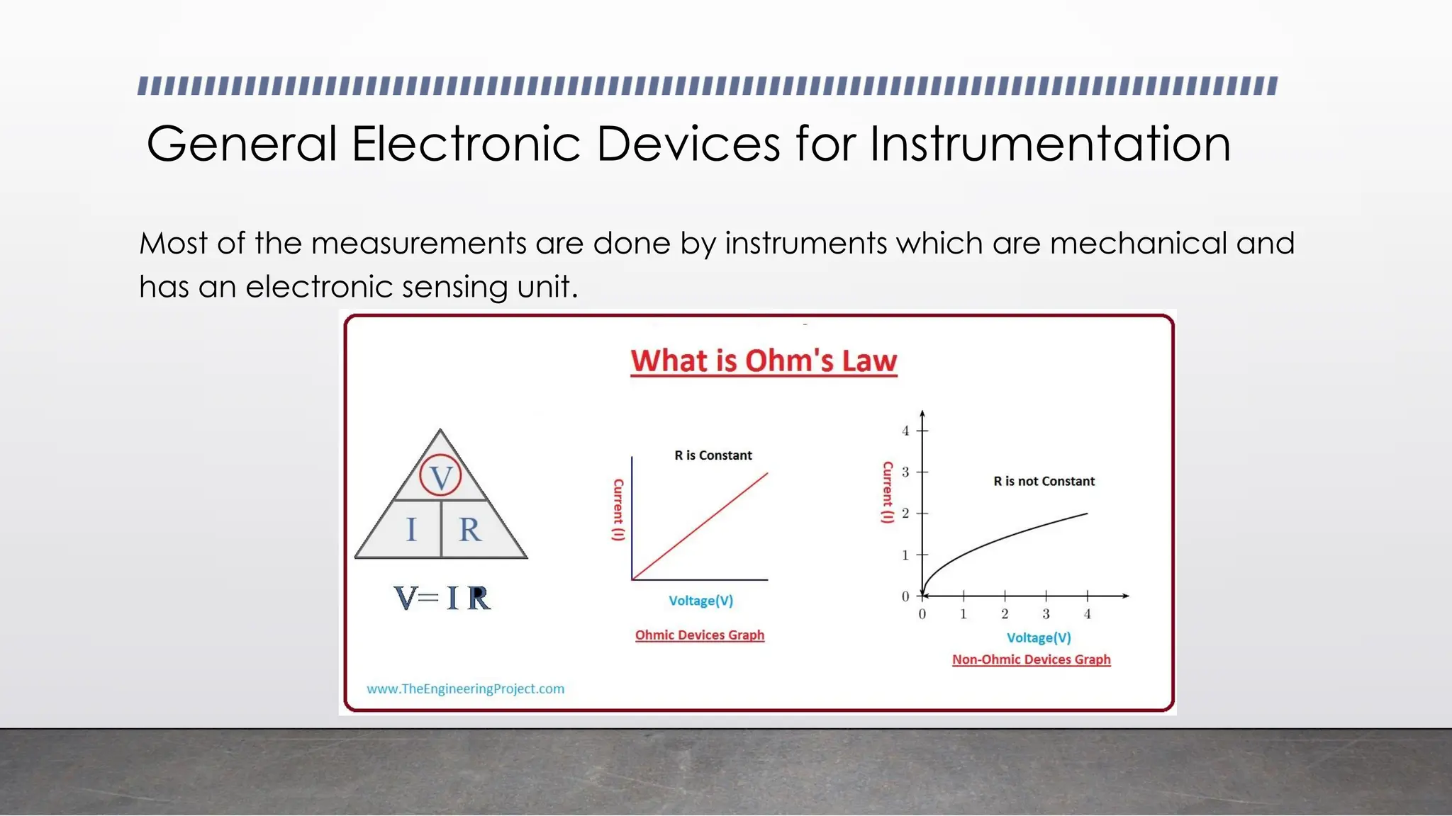
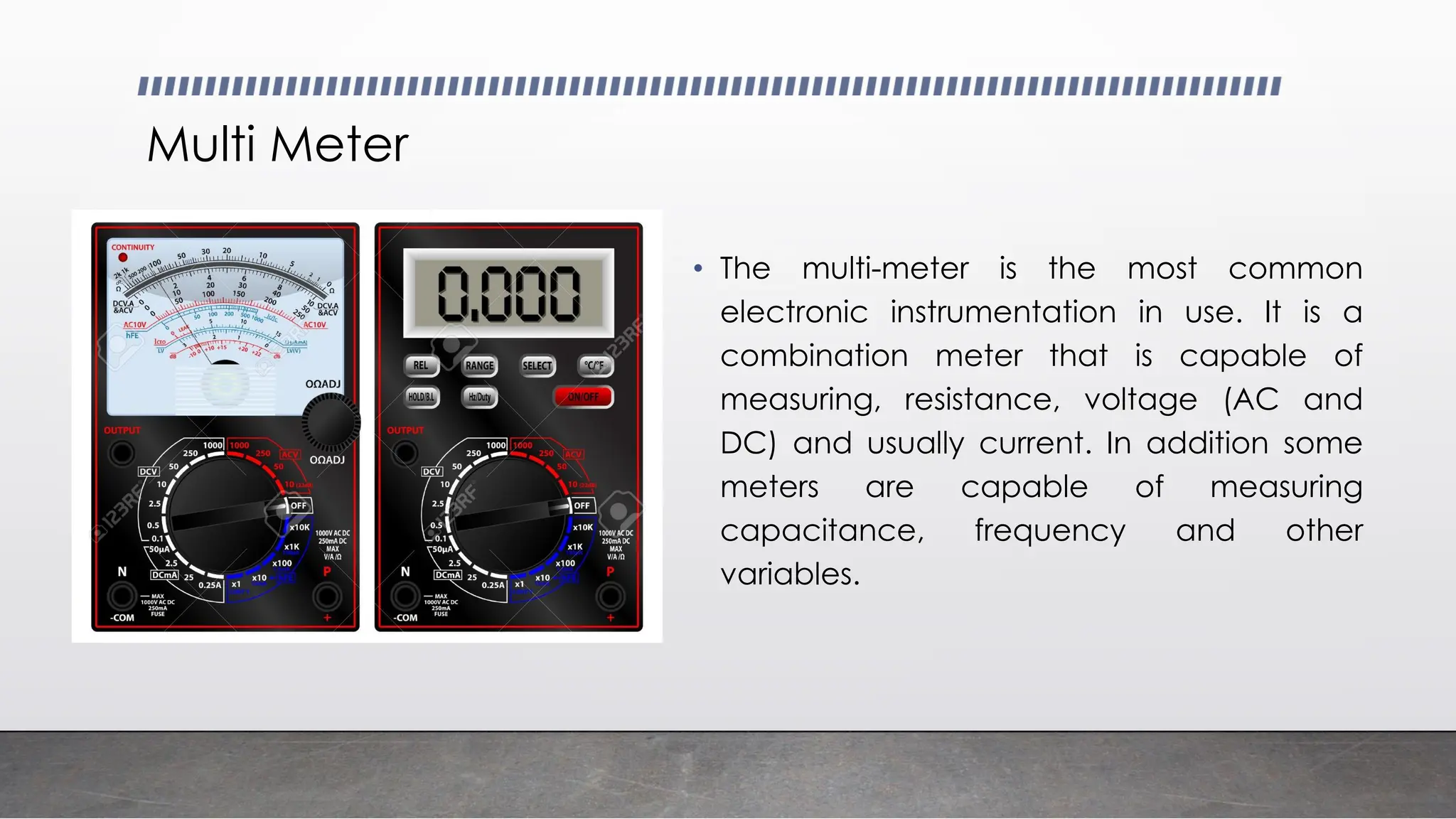
The document provides an overview of bio-instrumentation and control, focusing on electronic instruments' characteristics, divided into static and dynamic categories. It details performance metrics such as accuracy, precision, resolution, and drift for static characteristics, alongside speed of response, fidelity, and dynamic error for dynamic characteristics. Additionally, it describes various electronic devices used in instrumentation, including multimeters and oscilloscopes, outlining their functions and measurement capabilities.

1. Bio-instrumentation
and Control
Lecture 02- Introduction to General Electronic Instruments and
Characteristics

2. Characteristics of Instruments
• The performance characteristics of an instrument are mainly divided into
two categories:
i) Static characteristics
ii) Dynamic characteristics

3. Static Characteristics
The set of criteria defined for the instruments, which are used to measure the
quantities which are slowly varying with time or mostly constant, i.e., do not vary
with time, is called ‘static characteristics’.
i) Accuracy
ii) Precision
iii) Sensitivity
iv) Linearity
v) Reproducibility
vi) Repeatability
vii) Resolution
viii) Threshold
ix) Drift
x) Stability
xi) Tolerance
xii) Range or span

4. Accuracy
It is the degree of closeness with which the reading approaches the true value of the quantity
to be measured. The accuracy can be expressed in following ways:
a) Point accuracy:
Such accuracy is specified at only one particular point of scale. It does not give any
information about the accuracy at any other Point on the scale.
b) Accuracy as percentage of scale span:
When an instrument as uniform scale, its accuracy may be expressed in terms of scale range.
c) Accuracy as percentage of true value:
The best way to conceive the idea of accuracy is to specify it in terms of the true value of the
quantity being measured. (Precision)

5. Sensitivity
The sensitivity denotes the smallest
change in the measured variable to
which the instrument responds. It is
defined as the ratio of the changes in
the output of an instrument to a
change in the value of the quantity to
be measured.

6. Linearity
Ability to reproduce the input characteristics symmetrically and linearly.
X 100%

7. Reproducibility
It is the degree of closeness with which a given value may be repeatedly
measured. It is specified in terms of scale readings over a given period of
time.

8. Repeatability
It is defined as the variation of
scale reading & random in nature
Drift: Drift may be classified into
three categories:
a) zero drift:
If the whole calibration gradually
shifts due to slippage, permanent
set, or due to undue warming up
of electronic tube circuits, zero drift
sets in.

9. b) span drift or sensitivity drift
If there is proportional change in the indication all along the upward scale, the
drifts is called span drift or sensitivity drift.
c) Zonal drift:
In case the drift occurs only a portion of span of an instrument, it is called zonal
drift.

10. Resolution
If the input is slowly increased from some arbitrary input value, it will again be
found that output does not change at all until a certain increment is
exceeded. This increment is called resolution.

11. Threshold
If the instrument input is increased very gradually from zero there will be
some minimum value below which no output change can be detected. This
minimum value defines the threshold of the instrument.

12. Stability
It is the ability of an instrument to retain its performance throughout is
specified operating life.
The minimum & maximum values of a quantity for which an instrument is
designed to measure is called its range or span.
The Range or Span

13. Tolerance
The maximum allowable error in the measurement is specified in terms of
some value which is called tolerance.

14. Dynamic Characteristics
The set of criteria defined for the instruments, which are changes rapidly with time, is
called ‘dynamic characteristics.
The various static characteristics are:
i) Speed of response
ii) Measuring lag
iii) Fidelity
iv) Dynamic error

15. Speed of response: It is defined as the rapidity with which a measurement system responds to
changes in the measured quantity.
Measuring lag: It is the retardation or delay in the response of a measurement system to changes
in the measured quantity. The measuring lags are of two types:
a) Retardation type: In this case the response of the measurement system begins immediately
after the change in measured quantity has occurred.
b) Time delay lag: In this case the response of the measurement system begins after a dead time
after the application of the input.
Fidelity: It is defined as the degree to which a measurement system indicates changes in the
measurand quantity without dynamic error.
Dynamic error: It is the difference between the true value of the quantity changing with time &
the value indicated by the measurement system if no static error is assumed. It is also called
measurement error.

16. General Electronic Devices for Instrumentation
Most of the measurements are done by instruments which are mechanical and
has an electronic sensing unit.

17. Multi Meter
• The multi-meter is the most common
electronic instrumentation in use. It is a
combination meter that is capable of
measuring, resistance, voltage (AC and
DC) and usually current. In addition some
meters are capable of measuring
capacitance, frequency and other
variables.

18. 𝐴𝑐𝑡𝑢𝑎𝑙 𝑅𝑒𝑎𝑑𝑖𝑛𝑔 =
𝐹𝑢𝑙𝑙 𝑠𝑐𝑎𝑙𝑒 𝑟𝑎𝑛𝑔𝑒
𝑁𝑢𝑚𝑏𝑒𝑟 𝑜𝑓 𝑢𝑛𝑖𝑡𝑠
𝑋 𝑅𝑒𝑎𝑑𝑖𝑛𝑔

19. Use of multimeter in food industry
• To trouble shoot instruments; Food processing facilities often use a wide
variety of equipment. They could have pumps, mixers, valving equipment
and vacuum pumps on the process side; robotic package loaders on the
finishing side; as well as carton machines, automatic case packers and
conveyor systems. In these environments, maintenance technicians are
required to do multiple jobs, from checking out the robotics and PLC
programming, to fixing leading pumps and troubleshooting a vacuum
pump or automatic valve, among other applications and equipment.

20. 1. Voltage Measurement (V)
• Voltage measurements come in two flavors, AC and DC. These stand for
Alternating Current and Direct Current respectively.
DC
AC
In the world of AC waveforms
the effective voltage is called
the RMS voltage.

21. Peak Voltage - The voltage value at the local maximum point in the cycle
graph. The Voltage measure is from 0 to this maximum.
Peak to Peak Voltage – The Peak to Peak voltage is measured from the cycle
minimum value to the cycle maximum value. As an example if the ac waveform
below the P-P voltage would be 260 Volts (130 – (-130))
Average Voltage – The average voltage is the arithmatic average of the positive
half of the cycle. In a standard sinusoidal wave form this value is 0.637 * Peak
Voltage.
RMS or Effective Voltage – This is the Root-Mean-Square calculation of the
AC signal. This is the measure of how much work can be done by the AC power
source. The RMS value for a sinusoidal wave form is = .707 * Peak Voltage. For
non sinusoidal signals, the RMS value must be calculated.

22. Taking one cycle of AC signal and breaking it into
many small samples, you can calculate the RMS
value based on the following formula.
A meter that will break down the waveform into tiny
slices and make the mathematical RMS calculation
(above) and display the result of this calculation is
called a True RMS voltmeter. These meters will generate
an accurate RMS value for even non- symmetric
signals.

23. Resistance(R)
Resistance measurement is conducted by the same method in all meters. A fixed,
known current is applied to the resistance value that is being measured, and the
resulting voltage developed is used to quantify the resistance value.
The range of the resistance determines the amount of current applied. Lower
resistance values require higher current values to generate an accurately measurable
voltage. All resistance readings are made in Ohms, or multiples of Ohms (K- x1,000 M –
x1,000,000). In general readings above a few MegaOhms are considered to be open
circuits.
V = IR

24. Current (I)
• Reverse of the Resistance measurement.
• Field effect properties of currents flowing thru conductors

25. Frequency Counter
• Measures the amount of time it takes from one positive
going pulse to the next positive going pulse, and the result is
displayed as a number of cycles per second or Hertz.
• This function is built into some higher end hand held multi-
meters, but there are many more sophisticated bench top
frequency meters available.
• Most of these meters let you control exactly how you look
at the signal being measured.
• Common settings are weather the signal is triggered going
positive or going negative, and at what level this happens.
They may also let you look at the pulse period, positive
going portion or negative going pulse time, duty cycle and
other more advanced configurations involving two input
signals, such as time from the pulse on one channel to the
pulse on the other channel.

26. Function Generator
Function or frequency generators are a class of instrument that are useful for creating a repetitive signal
of a various form. In the mechanical world this is most commonly used to generate signals
to drive test apparatus.
There are two classes of function generator. The first is a standard signal generator that can create a
repetitive signal of a sine, triangle or square wave.
The second type of function generator is an arbitrary wave form generator. Used mostly by mechanical
engineers. The arbitrary wave form generator will allow you to program these complex waves, and then
play back these waveforms repeatedly.

27. • Frequency Control Section: The frequency section consists of a series of buttons (Labeled in BLUE) that select a course range setting,
and a dial (Labeled FREQ) that will is linearly adjustable for a fine adjust.
• Function Section: The function selection is a set of buttons (labeled in Red) that select between the a square wave, triangle wave and sine
wave output. This particular meter also includes a knob that allows the user to change the duty cycle from the standard 50% symmetry.
• Amplitude Section: The amplitude section controls the output amplitude of the wave form. Most frequency generators utilize a simple
vernier control knob for the output signal control. This vernier control adjusts the output level of the variable outputs from 0 to 100%.
• Output Section: The output section of the instrument actually outputs the signal that has been defined. Most output stages have at least
two outputs and possibly three. The two primary outputs you will find are an a 50Ohm output and a TTL or trigger output. The digital level
output provides a simple square wave output that matches the frequency of the settings. This is most commonly used to drive digital input
circuitry without fear of negative voltages destroying circuits.
The Attenuator selection is used to lower the maximum voltage of the output. This attenuator has selections for -20 db and – 40 db. This set
of buttons will allow you to set a maximum peak to peak voltage of 23V, 2.3V, 0.23V and 0.023V by selecting none, -20, -40 and both -20
and -40 respectively. This particular generator also has additional functions for triggering, and gating, which control when the signal is sent
and sweep, which is allowing the frequency to vary at a predetermined rate. This particular model also provides for a simple frequency
counter as described in section 2.0 by simply pushing a button.

28. Oscilloscope An oscilloscope is a laboratory instrument
commonly used to display and analyze the
waveform of electronic signals. In effect, the
device draws a graph of the instantaneous
signal voltage as a function of time.
A typical oscilloscope can display alternating
current (AC) or pulsating direct current (DC)
waveforms having a frequency as low as
approximately 1 hertz (Hz) or as high as
several megahertz (MHz).
High-end oscilloscopes can display signals
having frequencies up to several hundred
gigahertz (GHz). The display is broken up into
so-called horizontal divisions (hor div) and
vertical divisions (vert div).

29. Oscilloscope
• Time is displayed from left to right on the horizontal scale. Instantaneous voltage appears on the vertical scale,
with positive values going upward and negative values going downward.
• The oldest form of oscilloscope, still used in some labs today, is known as the cathode-ray oscilloscope. It
produces an image by causing a focused electron beam to travel, or sweep, in patterns across the face of a
cathode ray tube (CRT). More modern oscilloscopes electronically replicate the action of the CRT using a liquid
crystal display (liquid crystal display) similar to those found on notebook computers. The most sophisticated
oscilloscopes employ computers to process and display waveforms. These computers can use any type of
display, including CRT, LCD, and gas plasma.
• In any oscilloscope, the horizontal sweep is measured in seconds per division (s/div), milliseconds per division
(ms/div), microseconds per division (s/div), or nanoseconds per division (ns/div). The vertical deflection is
measured in volts per division (V/div), millivolts per division (mV/div), or microvolts per division (?V/div). Virtually all
oscilloscopes have adjustable horizontal sweep and vertical deflection settings