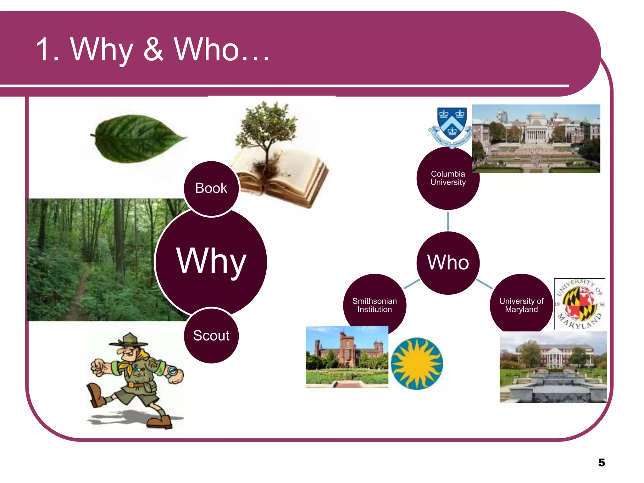
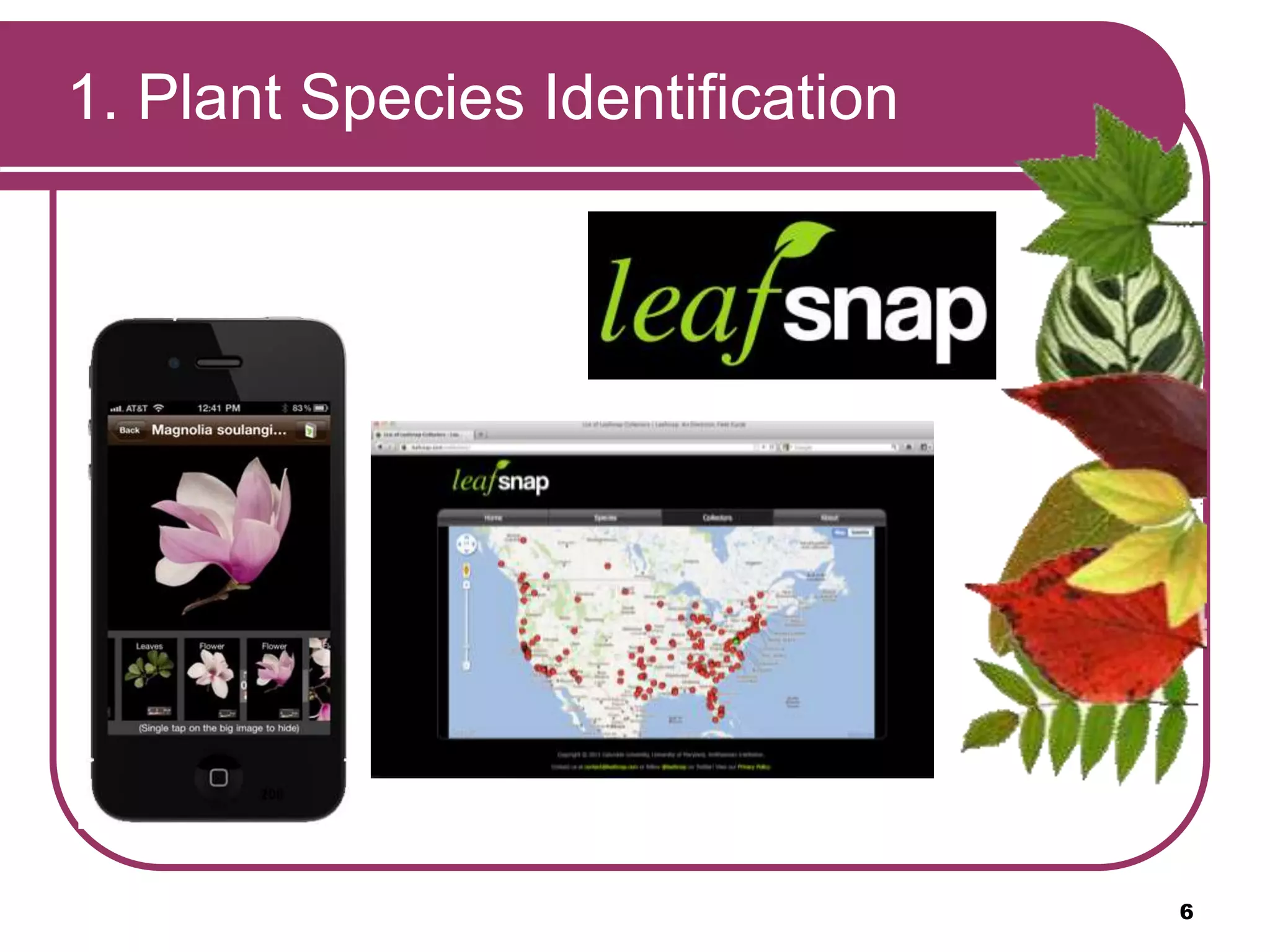
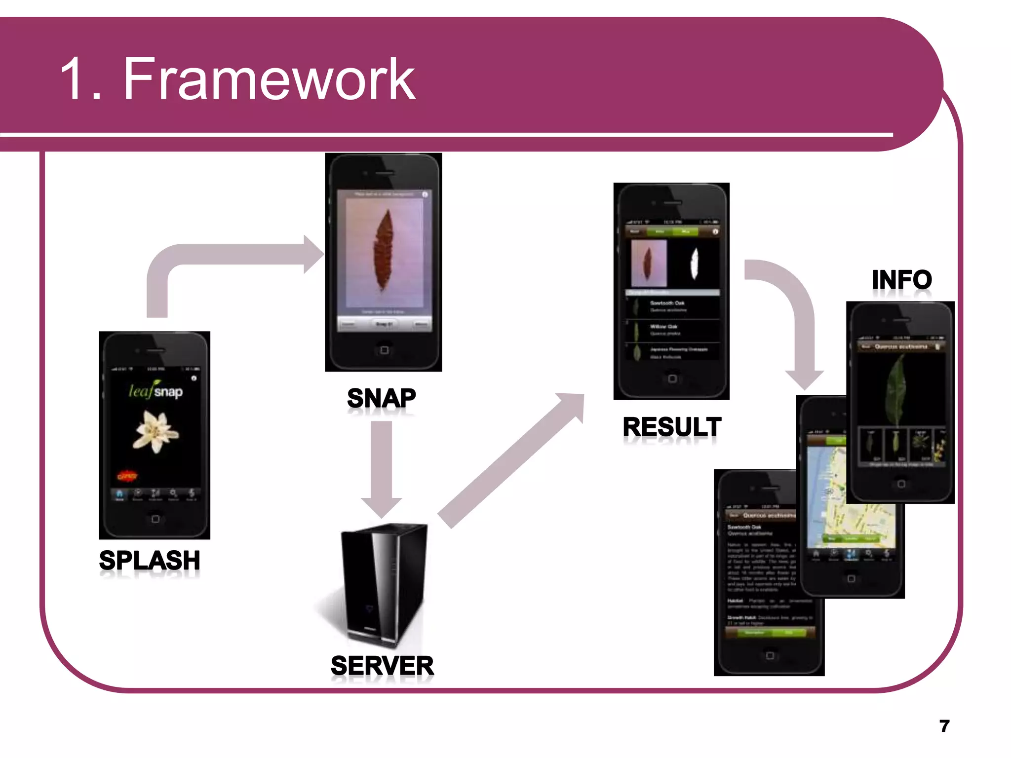
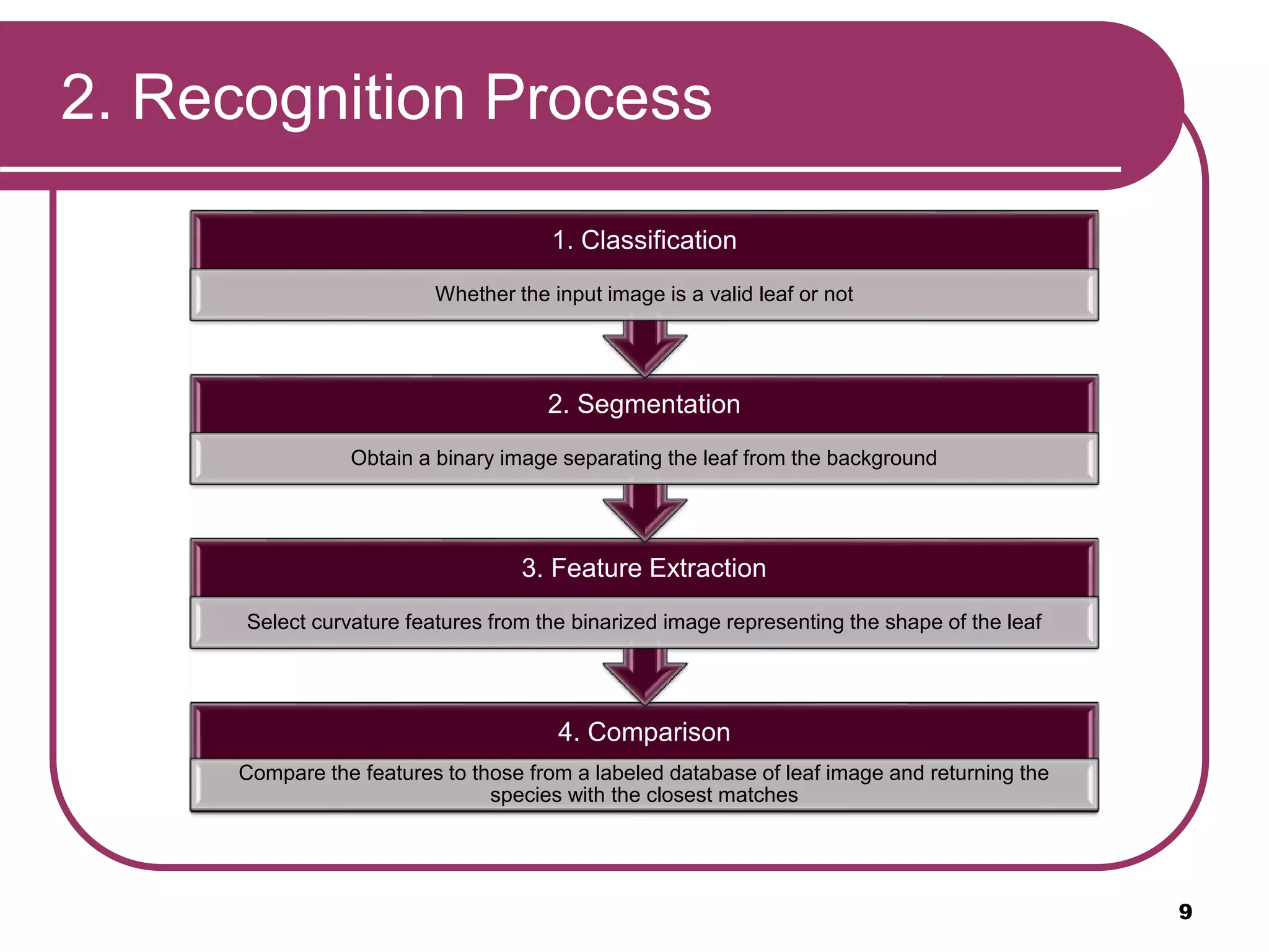
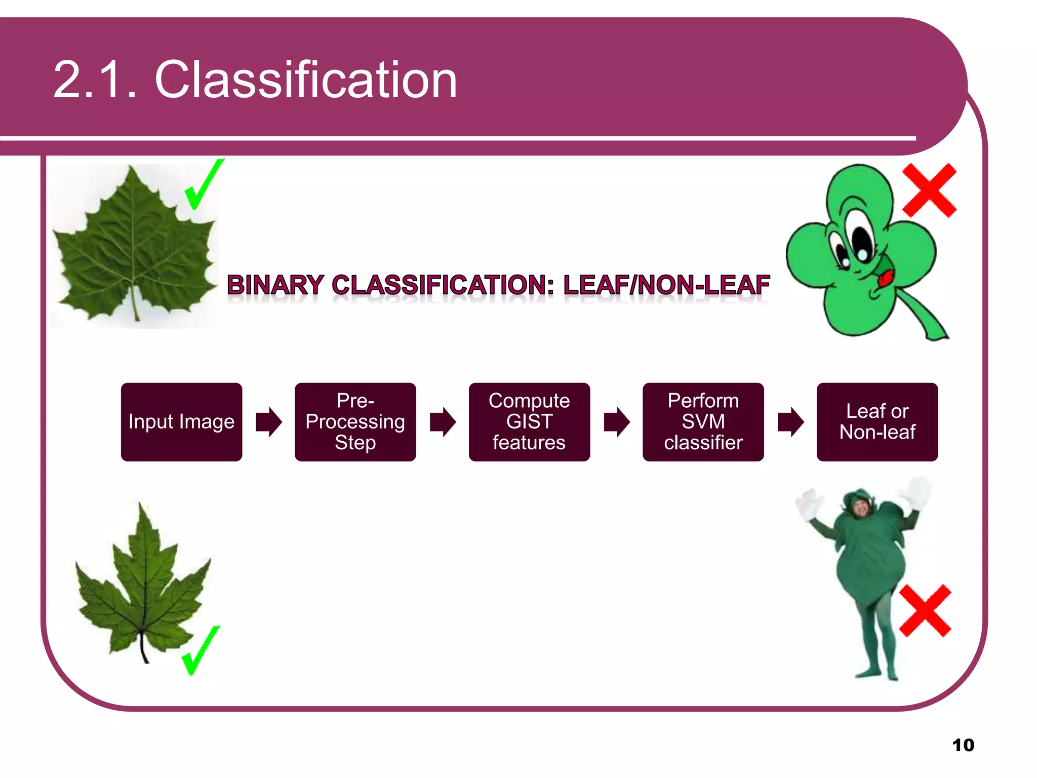
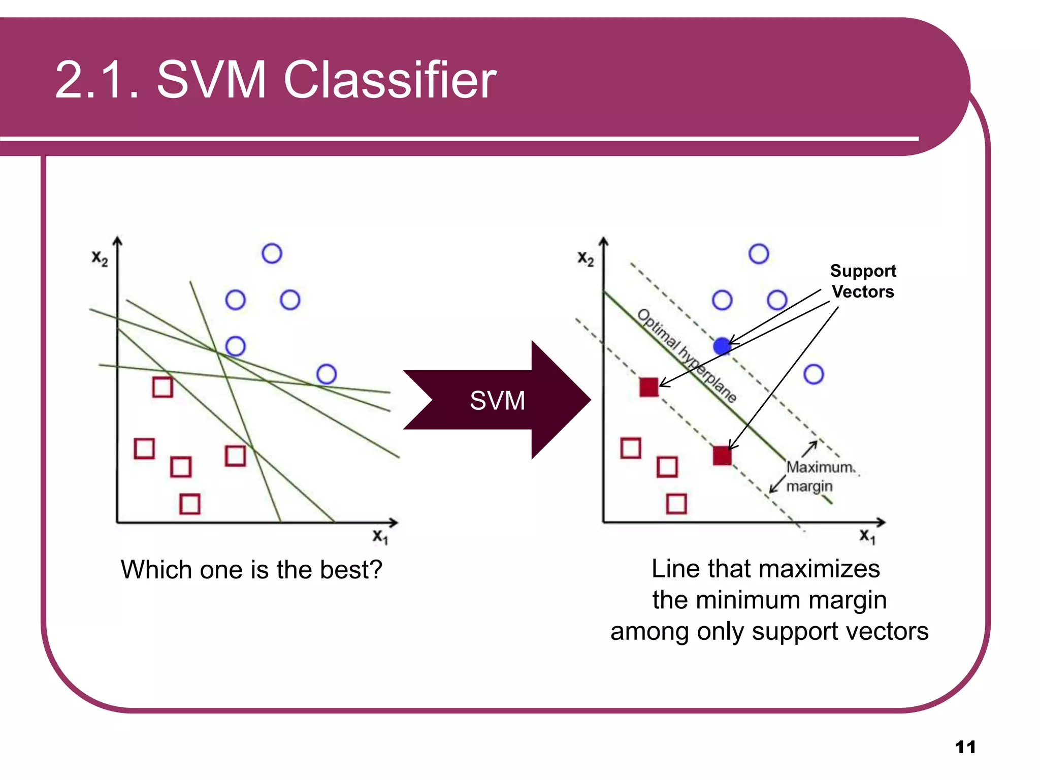
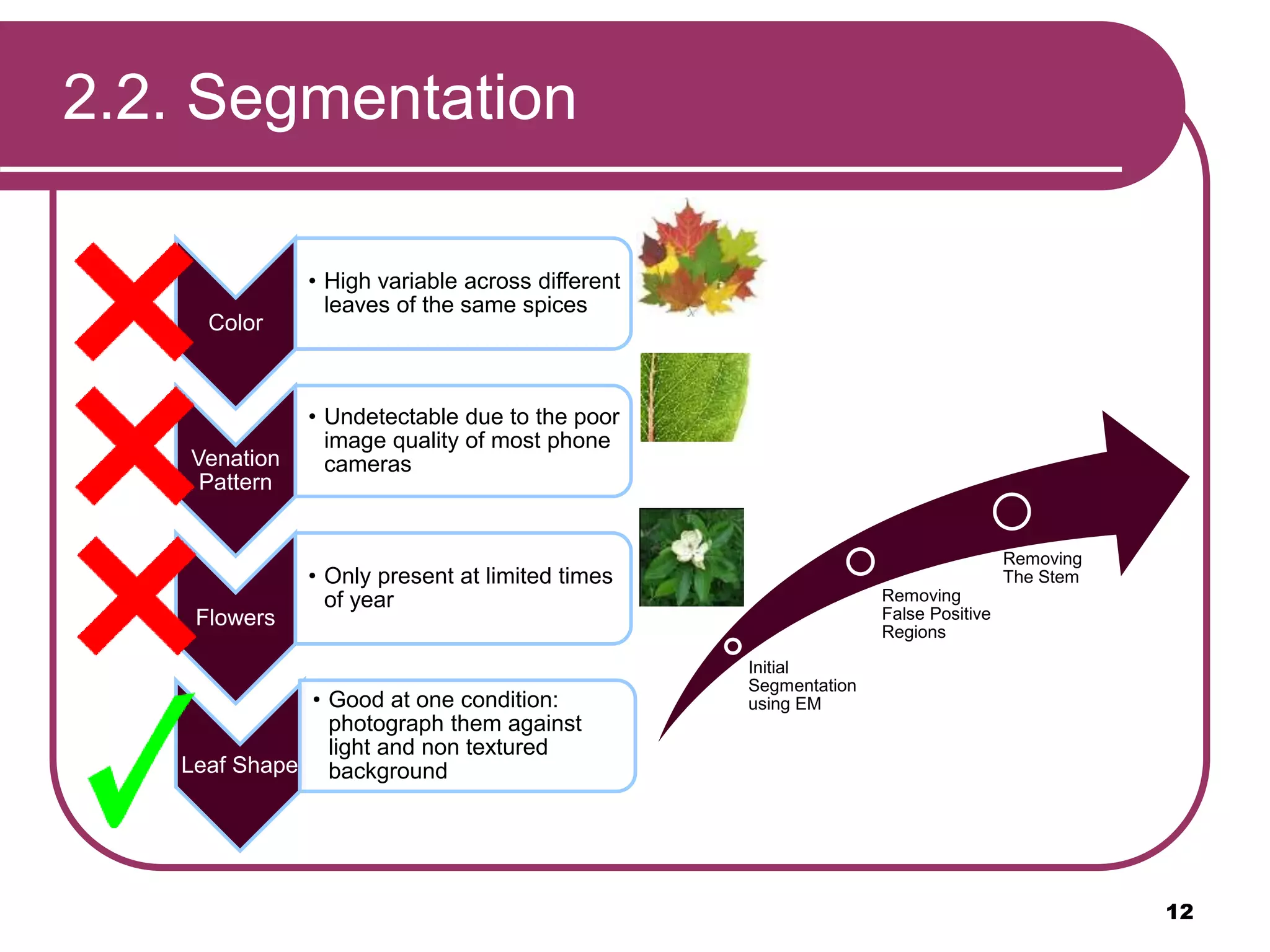
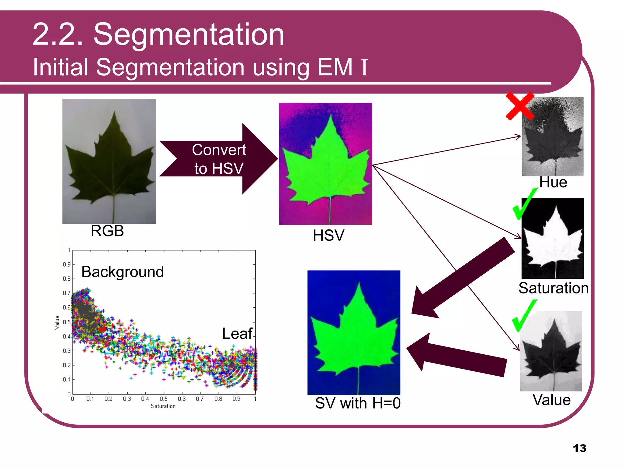
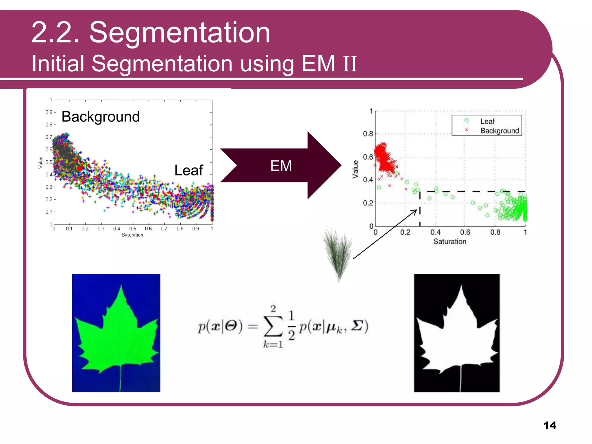
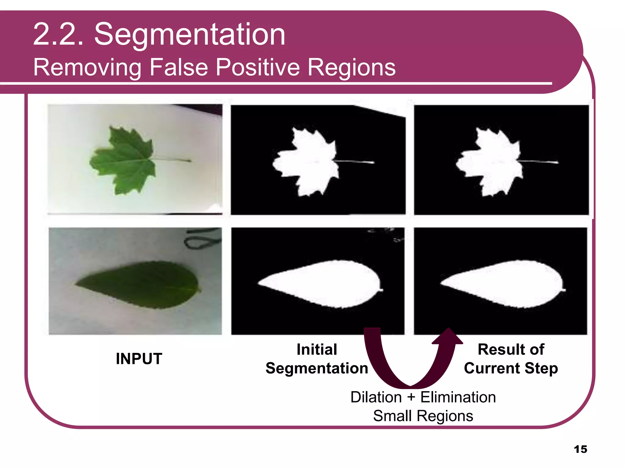
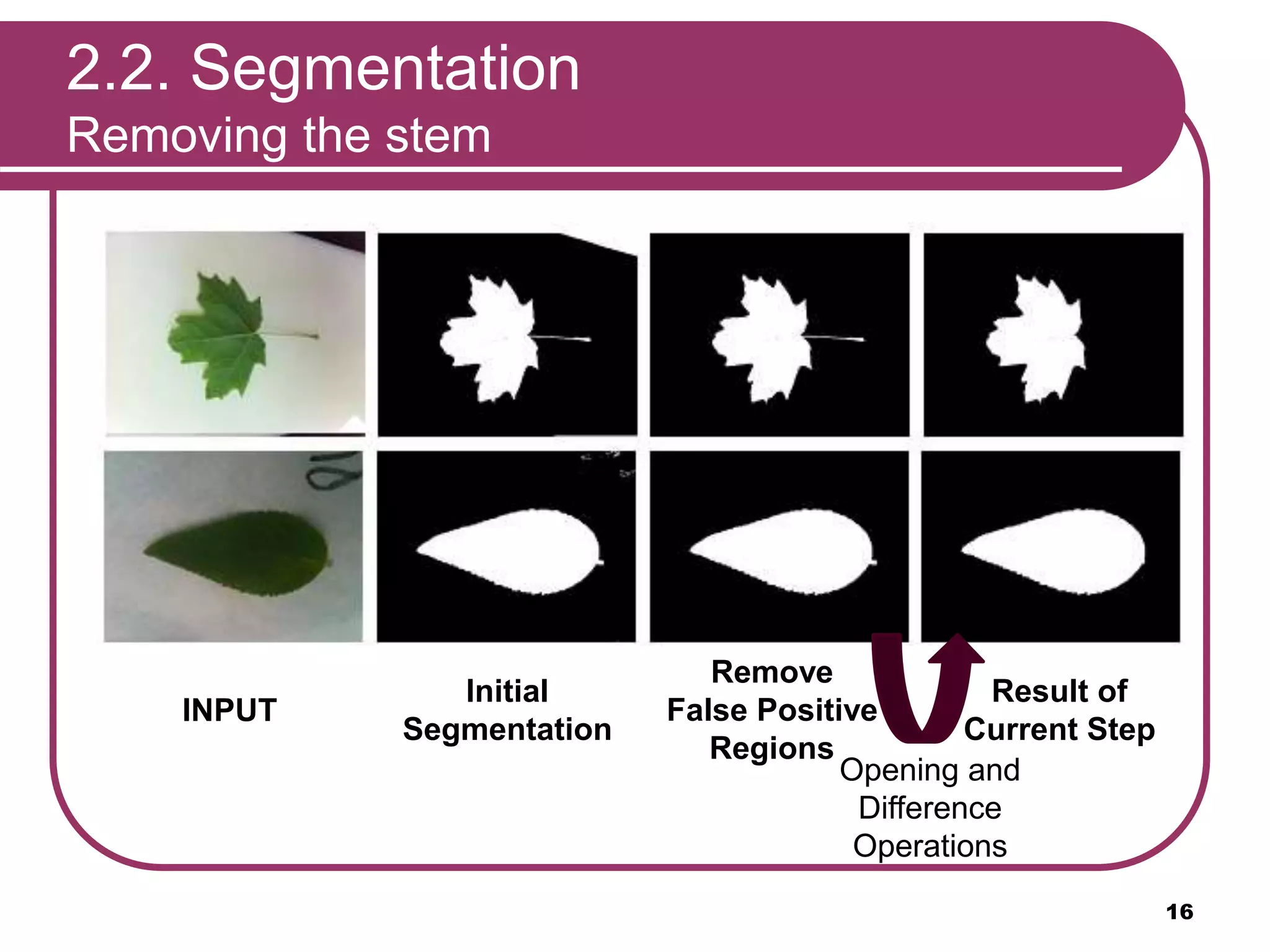
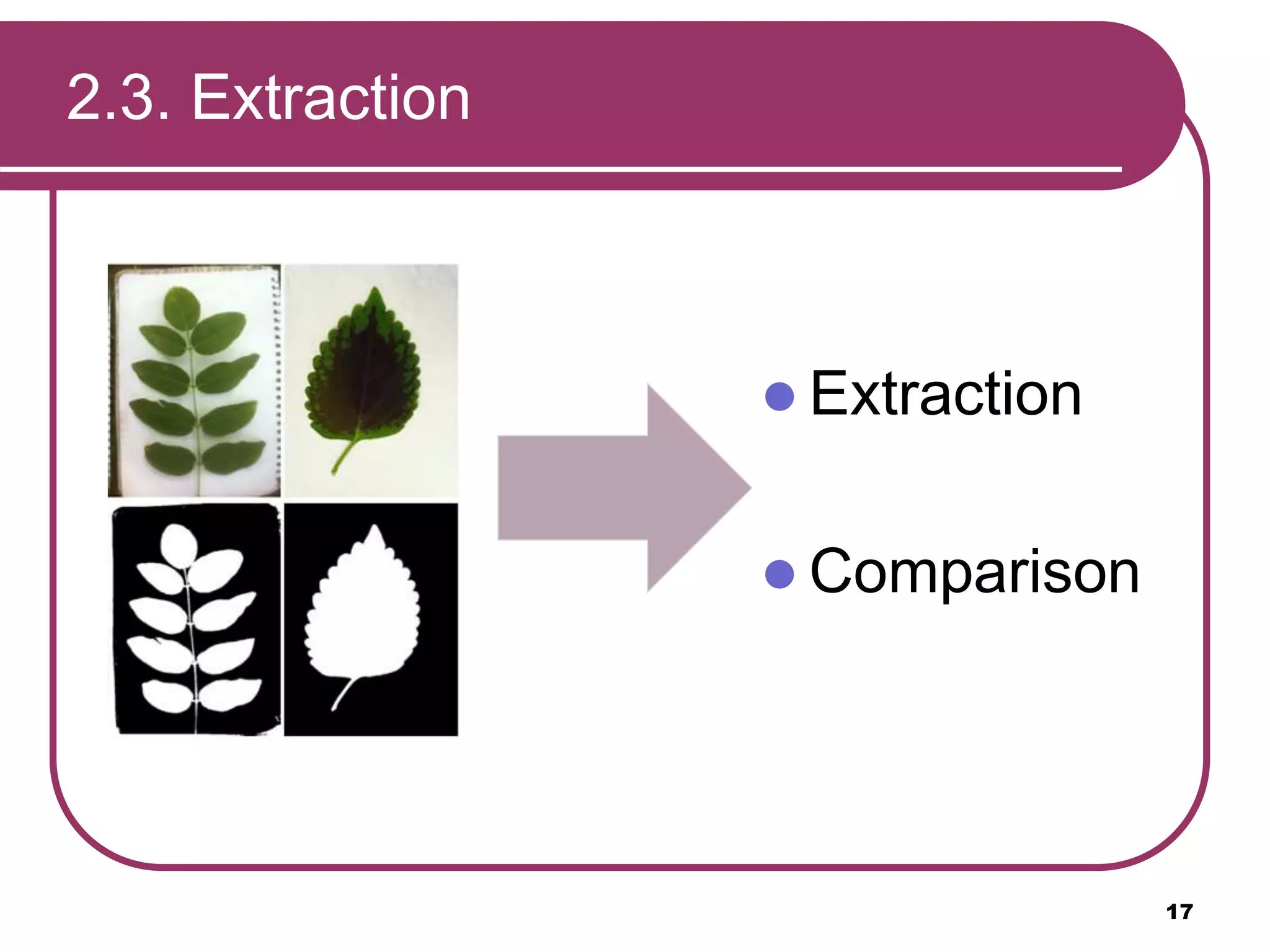
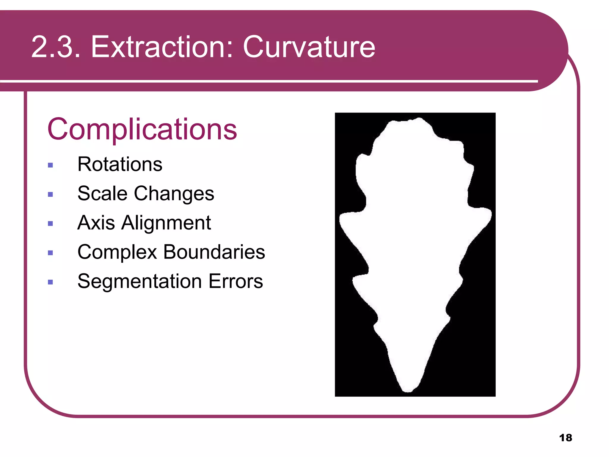
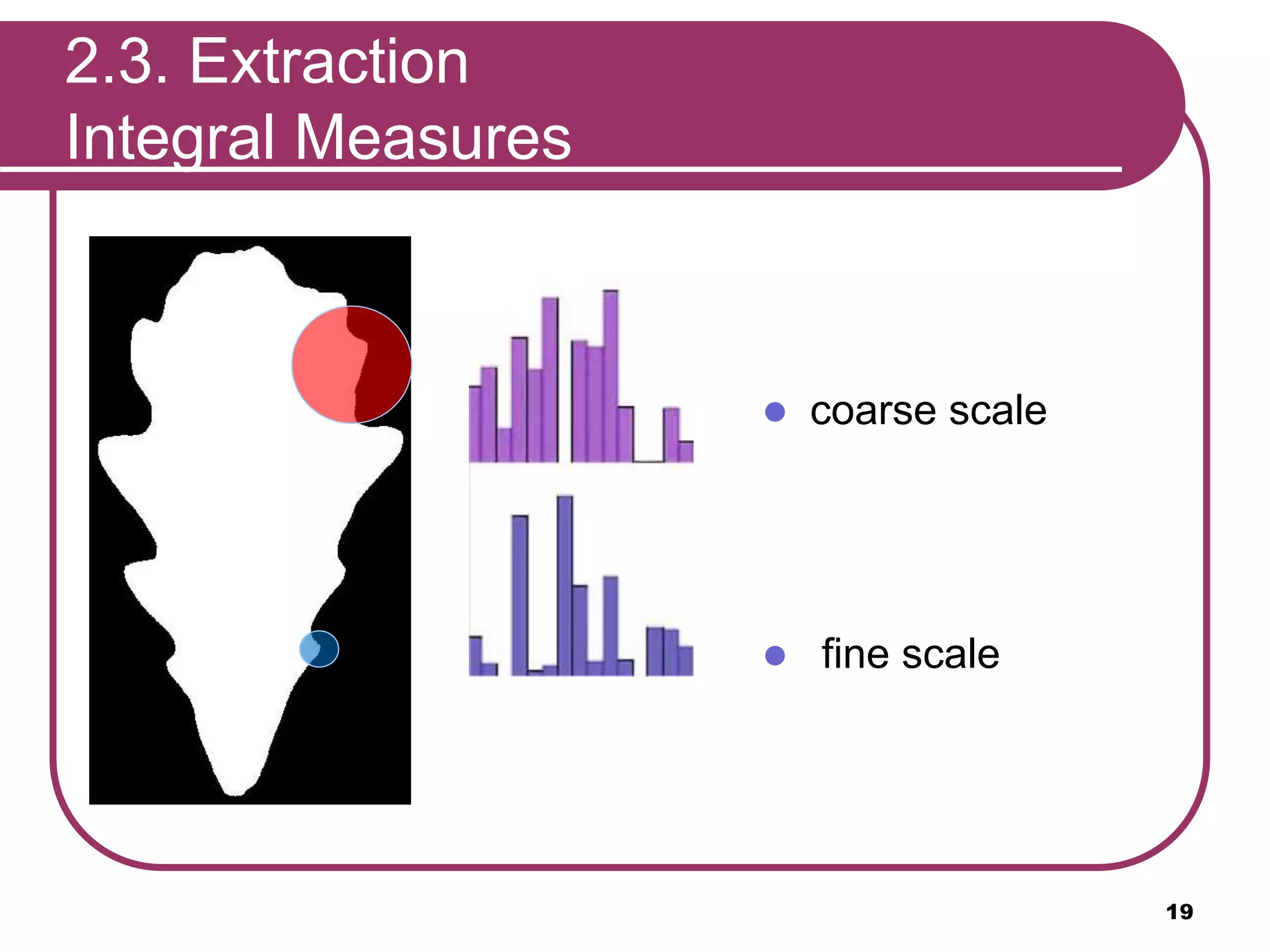
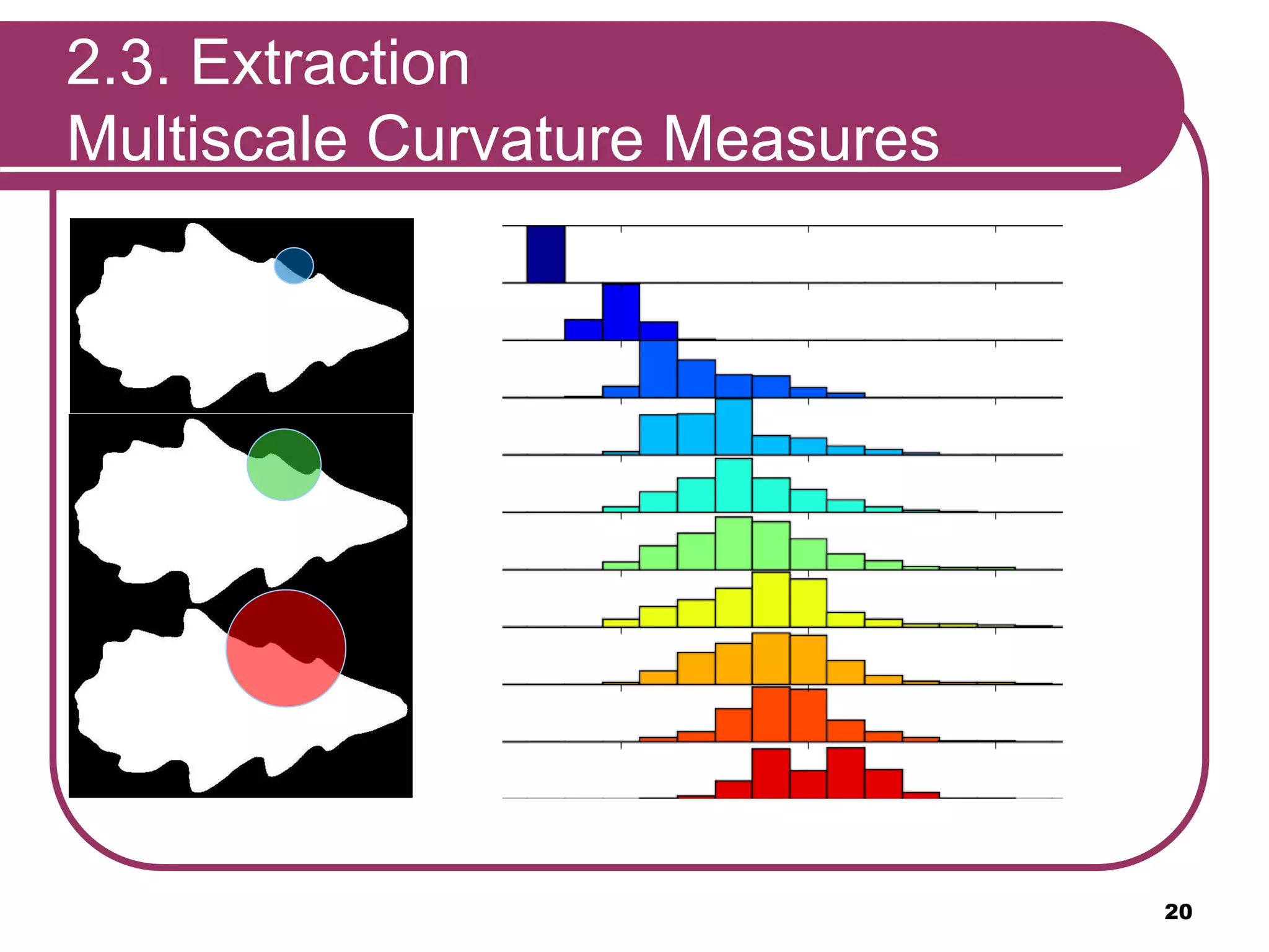
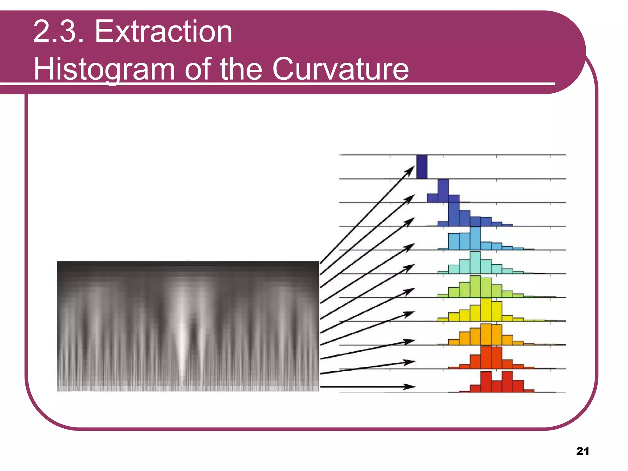
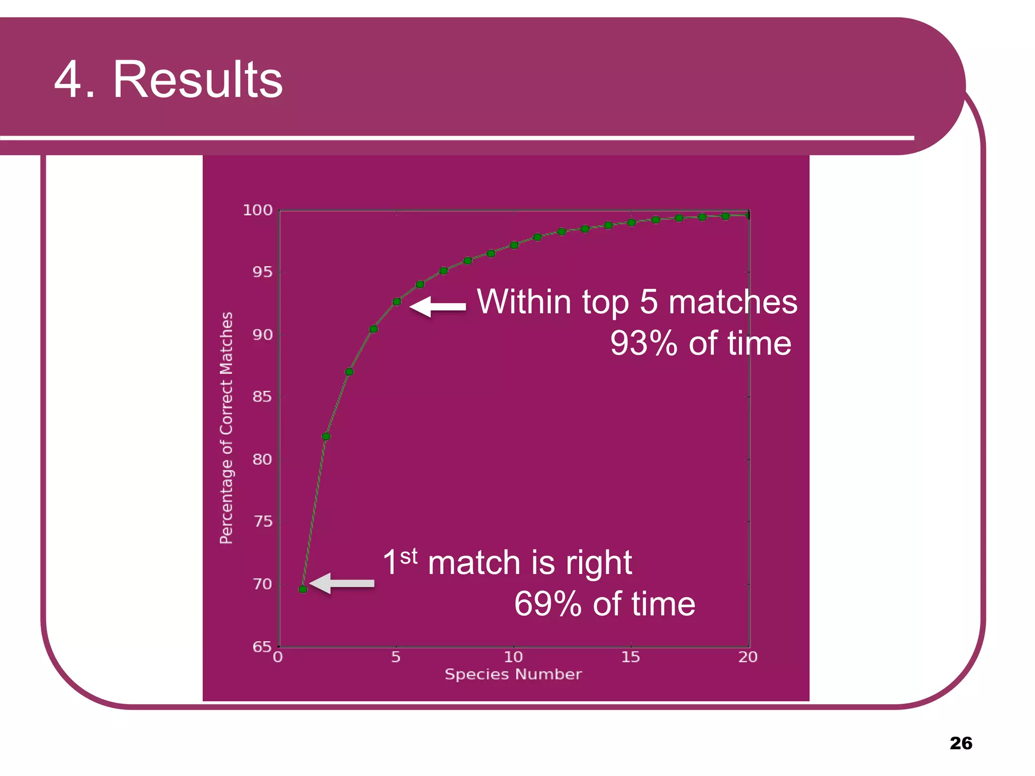
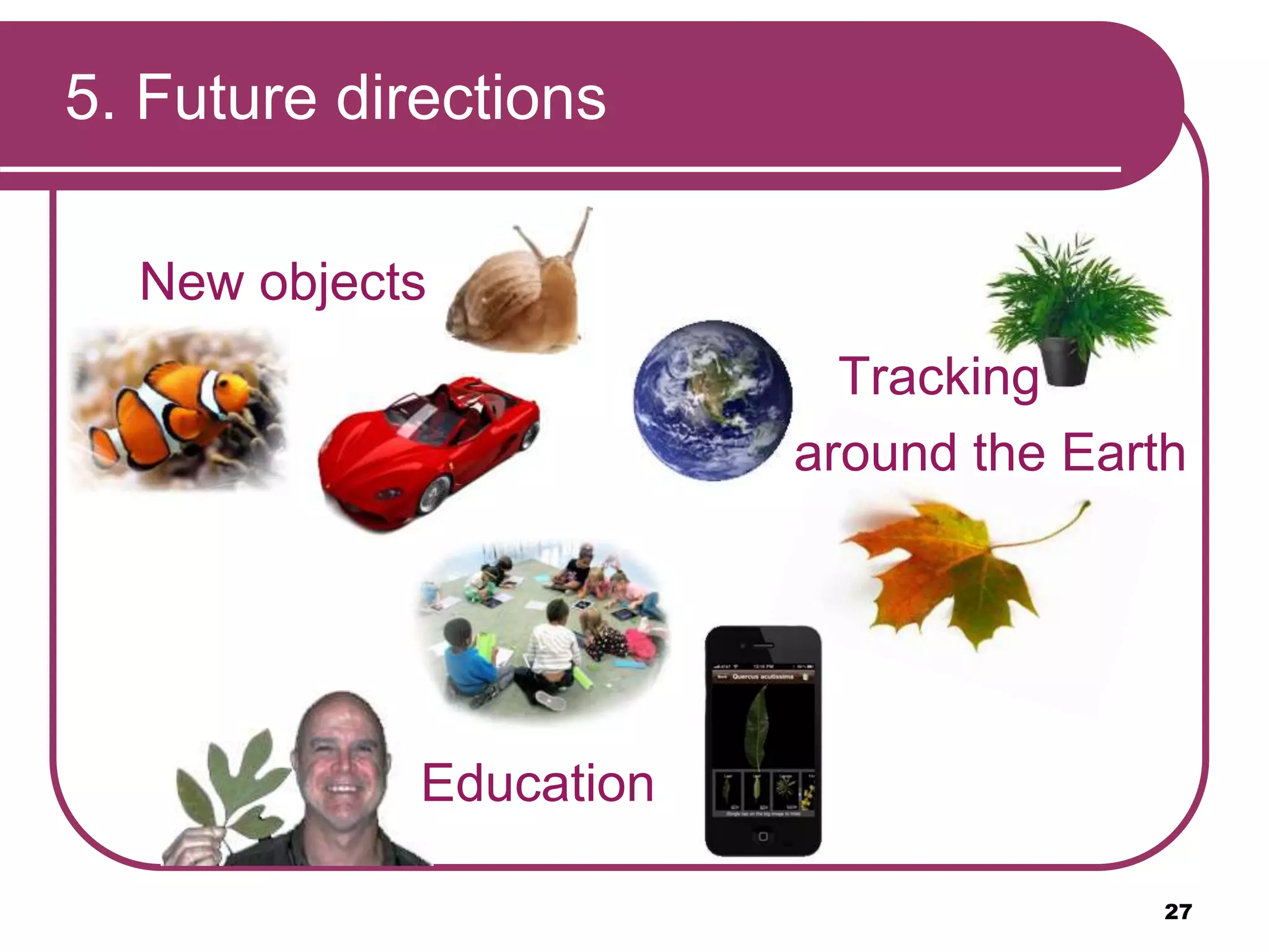
1
Leafsnap: classification
Mariia Dmitrieva
Mohamed Elawady
Paper
“Leafsnap: A Computer Vision System for Automatic
Plant Species Identification”
Neeraj Kumar, Peter N. Belhumeur, Arijit Biswas, David
W. Jacobs,W. John Kress, Ida C. Lopez, and Joao
V.B. Soares
European Conference on Computer Vision 2012
2
Outline
1.Introduction
2.Recognition Process
2.1. Classification
2.2. Segmentation
2.3. Feature Extraction
2.4. Comparison
4.Results
5.Future Directions
6.Demo
3
Outline
1.Introduction
2.Recognition Process
2.1. Classification
2.2. Segmentation
2.3. Feature Extraction
2.4. Comparison
4.Results
5.Future Directions
6.Demo
4
1. Why & Who…
5
Who
Columbia
University
University of
Maryland
Smithsonian
Institution
Why
Book
Scout
6
1. Plant Species Identification
7
1. Framework
Outline
1.Introduction
2.Recognition Process
2.1. Classification
2.2. Segmentation
2.3. Feature Extraction
2.4. Comparison
4.Results
5.Future Directions
6.Demo
8
2. Recognition Process
4. Comparison
Compare the features to those from a labeled database of leaf image and returning the
species with the closest matches
3. Feature Extraction
Select curvature features from the binarized image representing the shape of the leaf
2. Segmentation
Obtain a binary image separating the leaf from the background
1. Classification
Whether the input image is a valid leaf or not
9
2.1. Classification
Input Image
Pre-
Processing
Step
Compute
GIST
features
Perform
SVM
classifier
Leaf or
Non-leaf
10
2.1. SVM Classifier
11
Which one is the best?
Support
Vectors
SVM
Line that maximizes
the minimum margin
among only support vectors
2.2. Segmentation
Color
• High variable across different
leaves of the same spices
Venation
Pattern
• Undetectable due to the poor
image quality of most phone
cameras
Flowers
• Only present at limited times
of year
Leaf Shape
• Good at one condition:
photograph them against
light and non textured
background
Initial
Segmentation
using EM
Removing
False Positive
Regions
Removing
The Stem
12
2.2. Segmentation
Initial Segmentation using EM I
RGB
Convert
to HSV
HSV
HSV
Hue
HueSaturation
Saturation
Value
Value
SV
SV with H=0
Leaf
Background
13
2.2. Segmentation
Initial Segmentation using EM II
Leaf
Background
EM
SV
14
2.2. Segmentation
Removing False Positive Regions
INPUT
Initial
Segmentation
Result of
Current Step
Dilation + Elimination
Small Regions
15
2.2. Segmentation
Removing the stem
INPUT
Initial
Segmentation
Result of
Current Step
Opening and
Difference
Operations
Remove
False Positive
Regions
16
2.3. Extraction
17
 Extraction
 Comparison
2.3. Extraction: Curvature
Complications
 Rotations
 Scale Changes
 Axis Alignment
 Complex Boundaries
 Segmentation Errors
18
 coarse scale
 fine scale
19
2.3. Extraction
Integral Measures
20
2.3. Extraction
Multiscale Curvature Measures
2.3. Extraction
Histogram of the Curvature
21
2.3. Extraction
Advantages of the HoCS
 Fast
 Invariant to rotation
 Not requiring alignment
 Insensitive to small segmentation and
discretization errors
 Independent of the topological complexity
22
2.4. Comparison
 Nearest neighbors search
 Database:
 23,915 lab images
 5,129 mobile phone images
Broussonettia papyrifera
23
2.4. Comparison
Nearest neighbor search
 Comparison by histogram intersection distance:
 0.31 seconds
 Top 25 results are presented
24

B
i
ii baNbad ),min(),(
Outline
1.Introduction
2.Recognition Process
2.1. Classification
2.2. Segmentation
2.3. Feature Extraction
2.4. Comparison
4.Results
5.Future Directions
6.Demo
25
26
1st match is right
69% of time
Within top 5 matches
93% of time
4. Results
5. Future directions
New objects
27
Education
Tracking
around the Earth
6. Demo Video
28
Video By “Into Mobile”
http://www.youtube.com/watch?
v=k02C7p7mQ_c
Bibliography
 “Introduction to Support Vector Machines”
http://docs.opencv.org/doc/tutorials/ml/introduction_to_svm/introd
uction_to_svm.html
 “A Computer Vision System for Automatic Plant Species
Identification”
http://homes.cs.washington.edu/~neeraj/projects/leafsnap/base/pr
esentations/2012_leafsnap/leafsnap-eccv2012.pptx
 “Integral invariants for robust geometry processing” Pottmann, H.,
Wallner, J., Huang, Q.X., Yang, Y.L., Computer Aided Geometric
Design 26, 37–60 (2009)
29
30
Thanks For Listening !
Leafsnap: classification
31
QUESTIONS

Leafsnap: classification

Editor's Notes

  • #6 The Leafsnap is created to make a recognition of leaf plants easier for non-experts. The application was made in cooperation of teams from three different Universities: Columbia University, University of Maryland and Smithsonian Institution .
  • #7 There are a lot different plants in the earth, the application can recognize the leaf by the photo. The leafsnap is designed in USA and the database consists of the leafs for the Northeastern United States area.
  • #8 The framework consists of backend server and frontend mobile application. Backend server: accepts input images from end-users through mobile application, and sends back the top match results Frontend App: can be installed on iPad or iPhone (Android: still in progress) and have the following screens: Splash: home screen with picture randomly generated and stand for a few seconds in the beginning of app launch Snap: take a picture of the leaf for further uploading and processing Result: display the top matched leafs and let the end-user select the correct one according to corresponding info for each. Info: the final result can be represented in different ways (text, image, and map)
  • #10 To recognize a leaf, different characteristics can be used. In the application, the shape of the leaf is the basic for the identification process. The process and be considered in 4 steps: Classification -> Apply a binary classifier to the gist features Segmentation -> Estimate the foreground and background color distribution in the saturation-value space of the HSV color space Extraction -> Compute the histograms of curvature over multiple scales using integral measures of curvatures Comparison -> Use nearest neighbor approach with histogram intersection as distance metric
  • #11 How each step is done: Input Image -> Can be taken by mobile camera Pre-Processing Step -> resize the input image 300x400 and rotating it by 90 degrees if it has the wrong aspect ration (add scale-invariant property to GIST features). Compute GIST features -> Compute a set of perceptual features (naturalness, openness, roughness, expansion, ruggedness) that represent the dominant spatial structure of an image Perform SVM classifier -> Compute binary-based “support vector machine” classification algorithm with radial basis function as classification function Leaf or Non-leaf -> Output a binary result stating that the input image is qualified to be leaf or non-leaf image
  • #12 Reason: There exists multiple lines that offer a solution to the problem. Is any of them better than the others? We can intuitively define a criterion to estimate the worth of the lines Hint: A line is bad if it passes too close to the points because it will be noise sensitive and it will not generalize correctly. Therefore, our goal should be to find the line passing as far as possible from all points Support Vector Machine: finding the hyperplane which maximizes the margin of the training data (all data points) and minimize distance to the training examples (support vectors; subset of data points nearest to the hyperplane) If such linear decision surface does not exist, the data is mapped into a much higher dimensional space (“feature space”) where the separating decision surface is found
  • #13 Different parts can be used for the plant recognition, but the leaf is the best one. There are three steps for leaf segmentation from the background: (1) initial segmentation using expectation maximization method, (2) removing false positive regions, (3) removing the stem
  • #14 Hue is discarded because the background often has a greenish tinge due to reflections from the leaf or surrounding foliage
  • #15  The probability distribution of a pixel [x], represented by its saturation and value, is modeled as the sum of two Gaussians where each p(x|μk,Σ) is a Gaussian with mean μk and a common shared co-variance Σ Problem: Difficulty with pine leaves which have small part of leaves … same weight for each of the two Gaussians -> same number of pixels for each cluster Solution: define a rectangular region in saturation-value space that tends to contain leaf pixels … assign different weights to pixels inside and outside this region Two optimizations: one co-variance for both guassian functions, and estimation of gaussian parameters based on some part of image
  • #16  Reason: uneven background or shadows in the picture Where: outer border of the image Solution: dilation on segmented image + elimination of the connecting pixels on the image boundary
  • #17  Top-hat Transformation of segmentation: T_hat(B) = B − (B o S) Where B = Binary image resulting from last step (Remove False Positive Regions) S = Structure element (Disc with diameter larger than width of any stem in B) o = Opening morphological operation (erosion followed by dilation)
  • #18 Two stages of processing is done. The leaf is classified and segmented. So now we have binary image with the leaf’s pixels equal 1. Next stages are to extract the information about the curvature and compare it with the database.
  • #19 The curvature extraction is a sophisticated problem, there are a lot of complications, like rotation of the leaf on the image, scale changes, complex boundaries, problems of axis alignment and segmentation errors.
  • #20 To compute the curvature function integral measure is used. The idea is to measure the area of intersection of a circle centered at a contour point and the area inside of the contour. According to the measure the histogram can be constructed. Let’s consider a case with two radios of the circle, than there are 2 histograms for 2 different scales. The histograms of fine-scale values differ for each column and the coarse-scale values histograms differ for each row. The shape can be characterized by using both histograms together.
  • #21 In the approach described in the paper a lot of different radios are used. And as the result, there are the same number of the histogram. The name of the approach is Multiscale curvature measures.
  • #22 All the histograms are gathered together and result is presented on the slide. Radios is increasing from red diagram to the blue. And on the image the changing in values can be seen. The result is the HoCS feature, which is used to describe the specific shape of a leaf.
  • #23 The HoCS method has a lot of advantages. The main are: - Fast - Invariant to rotation - Not requiring alignment - Insensitive to small segmentation and discretization errors - Independent of the topological complexity
  • #24 When the HoCS feature is extracted, comparison (or identification) have to be done. For the purpose the nearest neighbors search is used. Database consist of 23,915 lab images and 5,129 mobile phone images. The difficult in the comparison small inter-species variation against the large intra-species. On the slide the different leaves of the same plant (Broussonettia papyrifera) are presented as an example.
  • #25 The histograms are normalized and compared using the formula (on the slide). B is the bin of the histogram (21 bins per scale of 525 values), N - feature dimensionality (25 scales). Then the result of the comparison is put into increasing order. The search takes only 0,31 seconds. And top 25 results are be presented to the user.
  • #27 To talk about an accuracy of the recognition, the resulted graph is presented. The first match in the rank is right in 69% of the cases, And in 93% of the cases user can find the right result in the top 5 matches.
  • #28 The recognition system can be extended in different aspects, applying for the other objects. The application can be used in education system, to study botanic for instance. The application widen its identification area from America to the other continents.