The document provides instructions for multiple activities involving interactive analysis and formatting of tables and charts in an e-fashion data universe. The activities include: 1) Creating tables and charts to analyze quantity sold by year and quarter, and formatting the header. 2) Formatting various chart types like column, surface line, and 3D pie charts using different styles and removing axes titles. 3) Formatting reports by adding sections, sums, breaks and page layout. 4) Defining the scope of analysis using a product lines hierarchy and adding rules to flag low and average performing product lines.

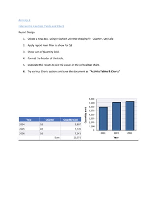
1. Activity 1
Interactive Analysis Table and Chart
Report Design
1. Create a new doc, using e-fashion universe showing Yr, Quarter , Qty Sold
2. Apply report level filter to show for Q1
3. Show sum of Quantity Sold.
4. Format the header of the table.
5. Duplicate the results to see the values in the vertical bar chart.
6. Try various Charts options and save the document as “Activity Tables & Charts“

2. Activity 2
Formatting Charts
1. Create a new query with Quantity Sold, State and Year
2. Add a query filter to the State object for California, Colorado and DC
3. Run the query
4. Get Column chart template from report element select region color as “Year”.
5. Format the Column chart as follows
a. Go to Format Chart >Global >General and Adjust the width as 11.08 cm and Height as
8.04 cm of the chart
b. Go to Legend properties and make legend visible.
c. Go to Format chart >Global >General and Remove the axis names State and Quantity
Sold(Category and Value axis)
d. Add Chart Title as Column Chart and make it visible
e. Give border to title
6. Add Border to chart
7. Copy the same Chart and apply Flashy styles to the chart.
8. Copy the same chart again and apply contrast style to it.
9. Copy the same chart and apply 3D- look to it.

3. 10. Insert a new report and create a Surface Line chart showing Quantity Sold by State and Year.
Select Year as a dimension and State as a region color. Format the chart as below
Adjust the Width as 11.08 cm and Height as 8.04 cm of the chart
Display the legend to the left of the chart (State)
Remove the axis Titles Year and Quantity Sold(secondary and value axis)
Show the data values in a Bold, dark blue and 10 point font size
Add a chart title of Surface Line Chart and make it into the centre and make it
visible.
Give border to title
11. Add Border to chart

4. 12. Insert a new report and create a 3d Pie Chart showing Quantity sold by Year. Format the chart
as follows.
Adjust the Width as 11.08 cm and Height as 8.04 cm of the chart
Show Quantity Sold data value on chart
Show segment label
Show the Quantity Sold data values as %
Remove Legends of Year
Create a chart background of dark grey color and Quantities Sold Chart data in White
Add a chart title of 3D Pie Chart
Change Background color of chart title to white.
Save the document as “ Activity Format Charts “

5. Activity 3
Formatting and Printing reports
1. Create a new doc showing State, Year, Quarter and Sales Revenue
2. Insert Section on Year and Quarter
3. Insert a sum total for each Quarter and Year using white text on a blue background
4. Insert a Column chart to show Sales Revenue by State at the level of Quarter
5. Save the document as “Formatting Reports “
6. Insert another report in the same document showing Sales Revenue by Quarter and Month
7. Insert a break on Year and Quarter
8. Format break of Year and Quarter
9. Insert a sum on Sales Revenue
10. At the report level, change the margins to 2 cm with a landscape page *
11. At the table level, format the alternating rows to display in light yellow
12. At the cell level, adjust the column widths of all columns. Display the YEAR value in bold red text
with a yellow background.
13. Insert another report in the same doc showing Year, Quarter, Month, Store name, State and
Sales Revenue
14. Click Page layout button to view how the report appears on the printer / PDF page.
15. Insert a break on the Year
16. For the Year column, select the option Avoid Page Breaks in table
17. Insert a section on State
18. At the section level, Select Start New Page for each state
19. Select the option Repeat on every new page for Year
20. Insert a break on Quarter and select the Avoid Page Breaks in table for Quarter

6. Activity 4
Analyzing the data
(Drillable doc by defining the scope of analysis in the report)
1. Create a new doc showing Product lines and Sales Revenue
2. Define the Scope of Analysis using the Product Lines hierarchy to display the following levels :
Category, SKU desc and Color
3. Create two Rule and define as follows
a. Add First Rule for value less the 500000, show that in red color which show low
performing lines.(Give Appropriate Name to rule)
b. Add second Rule for values greater then equal to 500000 and less the 3000000, show
data in blue color, which shows average performing lines. (Give Appropriate Name to
Rule)
4. Activate the Drill Mode to enable the Drill Down
5. Drill on the report to get the answers for low performing lines?