SlideShare a Scribd company logo
ECE 422 Session 7; Page 1/19
Power Flow Solutions
Power Flow Equations
In the system shown at right line models to have a
resistance of 0.01pu in addition to a series reactance of 0.1pu.
Bus 1
Bus 3
Bus 2
Bus 4
All branches have same series impedance:

pu 1

Zseries 0.01 j 0.1
 pu


Yseries
1
Zseries
 Yseries 0.99 9.901i

( ) pu


All branches have same shunt admittance (note that this is the value at each end, so it has

already been divided by 2).
Zshunt j
 10
 pu

Yshunt
1
Zshunt
 Yshunt 0.1i pu


Matrix elements:
y11 3 Yseries
 3Yshunt

 y33 2 Yseries
 2 Yshunt



y22 2 Yseries
 2Yshunt

 y44 3 Yseries
 3Yshunt


Ybus
y11
Yseries

Yseries

Yseries

Yseries

y22
0
Yseries

Yseries

0
y33
Yseries

Yseries

Yseries

Yseries

y44












 Ybus
2.97 29.403i

0.99
 9.901i

0.99
 9.901i

0.99
 9.901i

0.99
 9.901i

1.98 19.602i

0
0.99
 9.901i

0.99
 9.901i

0
1.98 19.602i

0.99
 9.901i

0.99
 9.901i

0.99
 9.901i

0.99
 9.901i

2.97 29.403i













pu


ECE 422 Session 7; Page 2/19
Reset origin for matrix and vector subscripts from 0 to 1. ORIGIN 1

Complex Form Equations:
S1 V1 V1

 Ybus
1 1


 V1 V2

 Ybus
1 2



 V1 V3

 Ybus
1 3



 V1 V4

 Ybus
1 4




=
S2 V2 V1

 Ybus
2 1


 V2 V2

 Ybus
2 2



 V2 V4

 Ybus
2 4




=
S3 V3 V1

 Ybus
3 1


 V3 V3

 Ybus
3 3



 V3 V4

 Ybus
3 4




=
S4 V4 V1

 Ybus
4 1


 V4 V2

 Ybus
4 2



 V4 V3

 Ybus
4 3



 V4 V4

 Ybus
4 4




=
Find real and imaginary parts of the Ybus matrix:
G Re Ybus
 
 G
2.97
0.99

0.99

0.99

0.99

1.98
0
0.99

0.99

0
1.98
0.99

0.99

0.99

0.99

2.97













B Im Ybus
 
 B
29.403

9.901
9.901
9.901
9.901
19.602

0
9.901
9.901
0
19.602

9.901
9.901
9.901
9.901
29.403














ECE 422 Session 7; Page 3/19
Rectangular Form
P1 V1
 2
G
1 1

 V1 V2
 G
1 2

cos θ1 θ2

( )
 B
1 2

sin θ1 θ2

( )


 

 V1 V3
 G
1 3

cos θ1 θ3

( )
 B
1 3

sin θ1 θ3

( )


 

 V1 V4
 G
1 4

cos θ1 θ4

( )
 B
1 4

sin θ1 θ4

( )





=
P2 V2 V1
 G
2 1

cos θ2 θ1

( )
 B
2 1

sin θ2 θ1

( )


 
 V2
 2
G
2 2


 V2 V4
 G
2 4

cos θ2 θ4

( )
 B
2 4

sin θ2 θ4

( )


 


=
P3 V3 V1
 G
3 1

cos θ3 θ1

( )
 B
3 1

sin θ3 θ1

( )


 
 V3
 2
G
3 3


 V3 V4
 G
3 4

cos θ3 θ4

( )
 B
3 4

sin θ3 θ4

( )


 


=
P4 V4 V1
 G
4 1

cos θ4 θ1

( )
 B
4 1

sin θ4 θ1

( )


 
 V4 V2
 G
4 2

cos θ4 θ2

( )
 B
4 2

sin θ4 θ2

( )


 

 V4 V3
 G
4 3

cos θ4 θ3

( )
 B
4 3

sin θ4 θ3

( )


 

 V4
 2
G
4


=
Q1 V1
 2
 B
1 1

 V1 V2
 G
1 2

sin θ1 θ2

( )
 B
1 2

cos θ1 θ2

( )


 

 V1 V3
 G
1 3

sin θ1 θ3

( )
 B
1 3

cos θ1 θ3

( )


 

 V1 V4
 G
1 4

sin θ1 θ4

( )
 B
1 4

cos θ1 
(





=
Q2 V2 V1
 G
2 1

sin θ2 θ1

( )
 B
2 1

cos θ2 θ1

( )


 
 V2
 2
B
2 2


 V2 V4
 G
2 4

sin θ2 θ4

( )
 B
2 4

cos θ2 θ4

( )


 


=
Q3 V3 V1
 G
3 1

sin θ3 θ1

( )
 B
3 1

cos θ3 θ1

( )


 
 V3
 2
B
3 3


 V3 V4
 G
3 4

sin θ3 θ4

( )
 B
3 4

cos θ3 θ4

( )


 


=
Q4 V4 V1
 G
4 1

sin θ4 θ1

( )
 B
4 1

cos θ4 θ1

( )


 
 V4 V2
 G
4 2

sin θ4 θ2

( )
 B
4 2

cos θ4 θ2

( )


 

 V4 V3
 G
4 3

sin θ4 θ3

( )
 B
4 3

cos θ4 θ3

( )


 

 V4
 2
B
4


=
You could plug the numbers for Gi,j and Bi,j into the equations next.
ECE 422 Session 7; Page 4/19
Newton-Raphson Example 1:
Reset origin for matrix and vector subscripts from 1 back to 0. ORIGIN 0

Use a simpler Ybus Ybus
j
 19.98

j 10

j 10

j 10

j
 19.98

j 10

j 10

j 10

j
 19.98










P2 0.5
 P3 1


Q2 0.5
 Q3 1


Slack Bus: V1m 1.0
 θ1 0

Initial Guesses: V2m0 1.0
 θ20 0

V3m0 1.0
 θ30 0

Power flow equations using initial guess:
P20 V2m0 V1m
 Im Ybus
1 0

 
 sin θ20 θ1

( )
 V2m0 V3m0
 Im Ybus
1 2

 
 sin θ20 θ30

( )



P30 V3m0 V1m
 Im Ybus
2 0

 
 sin θ30 θ1

( )
 V3m0 V2m0
 Im Ybus
2 1

 
 sin θ30 θ20

( )



Q20 V2m0
 V1m
 Im Ybus
1 0

 
 cos θ20 θ1

( )
 V2m0
2
Im Ybus
1 1

 

 V2m0 V3m0
 Im Ybus
1 2

 
 cos θ20 θ30

( )



Q30 V3m0
 V1m
 Im Ybus
2 0

 
 cos θ30 θ1

( )
 V3m0 V2m0
 Im Ybus
2 1

 
 cos θ30 θ20

( )

 V3m0
2
Im Ybus
2 2

 



Initial Mismatch Vector:
Use a "1-norm"
ΔH0
P2 P20

P3 P30

Q2 Q20

Q3 Q30













 ΔH0
0.5
1

0.52
0.98













 norm_1 out 0

out out ΔH0
x


x 0 3


for

norm_1 3
 well out of tolerance
ECE 422 Session 7; Page 5/19
Jacobian Terms
J11 submatrix
JP2θ2_0 Im Ybus
1 0

  V2m0
 V1m
 cos θ20 θ1

( )
 Im Ybus
1 2

  V2m0
 V3m0
 cos θ20 θ30

( )



JP2θ3_0 Im Ybus
1 2

 
 V2m0
 V3m0
 cos θ20 θ30

( )


JP3θ2_0 Im Ybus
2 1

 
 V3m0
 V2m0
 cos θ30 θ20

( )


JP3θ3_0 Im Ybus
2 0

  V3m0
 V1m
 cos θ30 θ1

( )
 Im Ybus
2 1

  V3m0
 V2m0
 cos θ30 θ20

( )



J12 submatrix
JP2Vm2_0 Im Ybus
1 0

  V1m
 sin θ20 θ1

( )
 Im Ybus
1 2

  V3m0
 sin θ20 θ30

( )



JP2Vm3_0 Im Ybus
1 2

  V2m0
 sin θ20 θ30

( )


JP3Vm2_0 Im Ybus
2 1

  V3m0
 sin θ30 θ20

( )


JP3Vm3_0 Im Ybus
2 0

  V1m
 sin θ30 θ1

( )
 Im Ybus
2 1

  V2m0
 sin θ30 θ20

( )



J21 submatrix
JQ2θ2_0 Im Ybus
1 0

  V2m0
 V1m
 sin θ20 θ1

( )
 Im Ybus
1 2

  V2m0
 V3m0
 sin θ20 θ30

( )



JQ2θ3_0 Im Ybus
1 2

 
 V2m0
 V3m0
 sin θ20 θ30

( )


JQ3θ2_0 Im Ybus
2 1

 
 V3m0
 V2m0
 sin θ30 θ20

( )


JQ3θ3_0 Im Ybus
2 0

  V3m0
 V1m
 sin θ30 θ1

( )
 Im Ybus
2 1

  V3m0
 V2m0
 sin θ30 θ20

( )



J22 submatrix
JQ2Vm2_0 Im Ybus
1 0

 
 V1m
 cos θ20 θ1

( )
 2 V2m0
 Im Ybus
1 1

 

 Im Ybus
1 2

  V3m0
 cos θ20 θ30

( )



JQ2Vm3_0 Im Ybus
1 2

 
 V2m0
 cos θ20 θ30

( )


JQ3Vm2_0 Im Ybus
2 1

 
 V3m0
 cos θ30 θ20

( )


JQ3Vm3_0 Im Ybus
2 0

 
 V1m
 cos θ30 θ1

( )
 Im Ybus
2 1

  V2m0
 cos θ30 θ20

( )

 2 V3m0
 Im Ybus
2 2

 



ECE 422 Session 7; Page 6/19
J_0
JP2θ2_0
JP3θ2_0
JQ2θ2_0
JQ3θ2_0
JP2θ3_0
JP3θ3_0
JQ2θ3_0
JQ3θ3_0
JP2Vm2_0
JP3Vm2_0
JQ2Vm2_0
JQ3Vm2_0
JP2Vm3_0
JP3Vm3_0
JQ2Vm3_0
JQ3Vm3_0












 J_0
20
10

0
0
10

20
0
0
0
0
19.96
10

0
0
10

19.96













Now solve for x (note, I'm using the built-in matrix inverse, but for a large case, one would use LU factorization
Δx1 J_0
1

ΔH0


Δx1
0
0.05

1.941 10
3


0.048














θ21 θ20 Δx1
0

 θ21 0 deg


θ31 θ30 Δx1
1

 θ31 2.865
 deg


V2m1 V2m0 Δx1
2

 V2m1 1.002

V3m1 V3m0 Δx1
3

 V3m1 0.952

Power flow equations using result of iteration 1:
P21 V2m1 V1m
 Im Ybus
1 0

 
 sin θ21 θ1

( )
 V2m1 V3m1
 Im Ybus
1 2

 
 sin θ21 θ31

( )



P31 V3m1 V1m
 Im Ybus
2 0

 
 sin θ31 θ1

( )
 V3m1 V2m1
 Im Ybus
2 1

 
 sin θ31 θ21

( )



Q21 V2m1
 V1m
 Im Ybus
1 0

 
 cos θ21 θ1

( )
 V2m1
2
Im Ybus
1 1

 

 V2m1 V3m1
 Im Ybus
1 2

 
 cos θ21 θ31

( )



Q31 V3m1
 V1m
 Im Ybus
2 0

 
 cos θ31 θ1

( )
 V3m1 V2m1
 Im Ybus
2 1

 
 cos θ31 θ21

( )

 V3m1
2
Im Ybus
2 2

 



ECE 422 Session 7; Page 7/19
Updated Mismatch Vector:
Use a "1-norm"
ΔH1
P2 P21

P3 P31

Q2 Q21

Q3 Q31













 ΔH1
0.023
0.048

0.013

0.071













 norm_11_NR out 0

out out ΔH1
x


x 0 3


for

good improvement
norm_11_NR 0.155

Jacobian Terms
J11 submatrix
JP2θ2_1 Im Ybus
1 0

  V2m1
 V1m
 cos θ21 θ1

( )
 Im Ybus
1 2

  V2m1
 V3m1
 cos θ21 θ31

( )



JP2θ3_1 Im Ybus
1 2

 
 V2m1
 V3m1
 cos θ21 θ31

( )


JP3θ2_1 Im Ybus
2 1

 
 V3m1
 V2m1
 cos θ31 θ21

( )


JP3θ3_1 Im Ybus
2 0

  V3m1
 V1m
 cos θ31 θ1

( )
 Im Ybus
2 1

  V3m1
 V2m1
 cos θ31 θ21

( )



J12 submatrix
JP2Vm2_1 Im Ybus
1 0

  V1m
 sin θ21 θ1

( )
 Im Ybus
1 2

  V3m1
 sin θ21 θ31

( )



JP2Vm3_1 Im Ybus
1 2

  V2m1
 sin θ21 θ31

( )


JP3Vm2_1 Im Ybus
2 1

  V3m1
 sin θ31 θ21

( )


JP3Vm3_1 Im Ybus
2 0

  V1m
 sin θ31 θ1

( )
 Im Ybus
2 1

  V2m1
 sin θ31 θ21

( )



J21 submatrix
JQ2θ2_1 Im Ybus
1 0

  V2m1
 V1m
 sin θ21 θ1

( )
 Im Ybus
1 2

  V2m1
 V3m1
 sin θ21 θ31

( )



JQ2θ3_1 Im Ybus
1 2

 
 V2m1
 V3m1
 sin θ21 θ31

( )


JQ3θ2_1 Im Ybus
2 1

 
 V3m1
 V2m1
 sin θ31 θ21

( )


JQ3θ3_1 Im Ybus
2 0

  V3m1
 V1m
 sin θ31 θ1

( )
 Im Ybus
2 1

  V3m1
 V2m1
 sin θ31 θ21

( )



ECE 422 Session 7; Page 8/19
J22 submatrix
JQ2Vm2_1 Im Ybus
1 0

 
 V1m
 cos θ21 θ1

( )
 2 V2m1
 Im Ybus
1 1

 

 Im Ybus
1 2

  V3m1
 cos θ21 θ31

( )



JQ2Vm3_1 Im Ybus
1 2

 
 V2m1
 cos θ21 θ31

( )


JQ3Vm2_1 Im Ybus
2 1

 
 V3m1
 cos θ31 θ21

( )


JQ3Vm3_1 Im Ybus
2 0

 
 V1m
 cos θ31 θ1

( )
 Im Ybus
2 1

  V2m1
 cos θ31 θ21

( )

 2 V3m1
 Im Ybus
2 2

 



J_1
JP2θ2_1
JP3θ2_1
JQ2θ2_1
JQ3θ2_1
JP2θ3_1
JP3θ3_1
JQ2θ3_1
JQ3θ3_1
JP2Vm2_1
JP3Vm2_1
JQ2Vm2_1
JQ3Vm2_1
JP2Vm3_1
JP3Vm3_1
JQ2Vm3_1
JQ3Vm3_1












 J_1
19.545
9.525

0.477
0.477
9.525

19.032
0.477

0.952

0.476
0.476

20.531
9.507

0.501
1.001

10.007

18.043













Now solve for x
Δx2 J_1
1

ΔH1


Δx2
2.542 10
5


2.894
 10
3


3.621
 10
3


5.998
 10
3



















θ22 θ21 Δx2
0

 θ22 1.457 10
3

 deg


θ32 θ31 Δx2
1

 θ32 3.031
 deg


V2m2 V2m1 Δx2
2

 V2m2 0.998

V3m2 V3m1 Δx2
3


V3m2 0.946

ECE 422 Session 7; Page 9/19
Power flow equations using result of iteration 2:
P22 V2m2 V1m
 Im Ybus
1 0

 
 sin θ22 θ1

( )
 V2m2 V3m2
 Im Ybus
1 2

 
 sin θ22 θ32

( )



P32 V3m2 V1m
 Im Ybus
2 0

 
 sin θ32 θ1

( )
 V3m2 V2m2
 Im Ybus
2 1

 
 sin θ32 θ22

( )



Q22 V2m2
 V1m
 Im Ybus
1 0

 
 cos θ22 θ1

( )
 V2m2
2
Im Ybus
1 1

 

 V2m2 V3m2
 Im Ybus
1 2

 
 cos θ22 θ32

( )



Q32 V3m2
 V1m
 Im Ybus
2 0

 
 cos θ32 θ1

( )
 V3m2 V2m2
 Im Ybus
2 1

 
 cos θ32 θ22

( )

 V3m2
2
Im Ybus
2 2

 



Updated Mismatch Vector:
Use a "1-norm"
ΔH2
P2 P22

P3 P32

Q2 Q22

Q3 Q32













 ΔH2
2.672 10
4


4.417
 10
4


7.148
 10
5


5.592
 10
4


















 norm_12_FD out 0

out out ΔH2
x


x 0 3


for

norm_12_FD 1.34 10
3


 close to a desirable tolerance
Find P and Q at slack bus:
P1 V1m V2m2
 Im Ybus
0 1

 
 sin θ1 θ22

( )
 V1m V3m2
 Im Ybus
0 2

 
 sin θ1 θ32

( )



P1 0.5
 P1 P2
 1

Q1 V1m
2
 Im Ybus
0 0

 
 V2m2 Im Ybus
0 1

 
 cos θ1 θ22

( )

 V1m V3m2
 Im Ybus
0 2

 
 cos θ1 θ32

( )



Q1 0.551
 Q1 Q22
 1.051

ECE 422 Session 7; Page 10/19
Newton-Raphson Example 2:
Now suppose that we were given that the voltage at bus 2 is know (voltage regulated bus):
V2m 1.02

Now V2m is no longer an unknown, which reduces the size of the problem to solve
Power flow equations using initial guess:
P20 V2m V1m
 Im Ybus
1 0

 
 sin θ20 θ1

( )
 V2m V3m0
 Im Ybus
1 2

 
 sin θ20 θ30

( )



P30 V3m0 V1m
 Im Ybus
2 0

 
 sin θ30 θ1

( )
 V3m0 V2m
 Im Ybus
2 1

 
 sin θ30 θ20

( )



Q2 equation is no longer needed here
Q30 V3m0
 V1m
 Im Ybus
2 0

 
 cos θ30 θ1

( )
 V3m0 V2m
 Im Ybus
2 1

 
 cos θ30 θ20

( )

 V3m0
2
Im Ybus
2 2

 



Initial Mismatch Vector:
Use a "1-norm"
ΔH0
P2 P20

P3 P30

Q3 Q30









 ΔH0
0.5
1

0.78









 norm_1 out 0

out out ΔH0
x


x 0 2


for

norm_1 2.28
 well out of tolerance
Jacobian Terms
J11 submatrix
JP2θ2_0 Im Ybus
1 0

  V2m
 V1m
 cos θ20 θ1

( )
 Im Ybus
1 2

  V2m
 V3m0
 cos θ20 θ30

( )



JP2θ3_0 Im Ybus
1 2

 
 V2m
 V3m0
 cos θ20 θ30

( )


JP3θ2_0 Im Ybus
2 1

 
 V3m0
 V2m
 cos θ30 θ20

( )


JP3θ3_0 Im Ybus
2 0

  V3m0
 V1m
 cos θ30 θ1

( )
 Im Ybus
2 1

  V3m0
 V2m
 cos θ30 θ20

( )



ECE 422 Session 7; Page 11/19
J12 submatrix (no longer have partials with respect to V2m)
JP2Vm3_0 Im Ybus
1 2

  V2m
 sin θ20 θ30

( )


JP3Vm3_0 Im Ybus
2 0

  V1m
 sin θ30 θ1

( )
 Im Ybus
2 1

  V2m
 sin θ30 θ20

( )



J21 submatrix (no longer have Q2 terms)
JQ3θ2_0 Im Ybus
2 1

 
 V3m0
 V2m
 sin θ30 θ20

( )


JQ3θ3_0 Im Ybus
2 0

  V3m0
 V1m
 sin θ30 θ1

( )
 Im Ybus
2 1

  V3m0
 V2m
 sin θ30 θ20

( )



J22 submatrix
JQ2Vm3_0 Im Ybus
1 2

 
 V2m
 cos θ20 θ30

( )


JQ3Vm3_0 Im Ybus
2 0

 
 V1m
 cos θ30 θ1

( )
 Im Ybus
2 1

  V2m
 cos θ30 θ20

( )

 2 V3m0
 Im Ybus
2 2

 



J_0
JP2θ2_0
JP3θ2_0
JQ3θ2_0
JP2θ3_0
JP3θ3_0
JQ3θ3_0
JP2Vm3_0
JP3Vm3_0
JQ3Vm3_0








 J_0
20.4
10.2

0
10.2

20.2
0
0
0
19.76









Now solve for x (note, I'm using the built-in matrix inverse, but for a large case, we would use LU factorization
Δx1 J_0
1

ΔH0


Δx1
3.246
 10
4


0.05

0.039












θ21 θ20 Δx1
0

 θ21 0.019
 deg


θ31 θ30 Δx1
1

 θ31 2.846
 deg


V3m1 V3m0 Δx1
2


V3m1 0.961

ECE 422 Session 7; Page 12/19
Power flow equations using result of iteration 1:
P21 V2m V1m
 Im Ybus
1 0

 
 sin θ21 θ1

( )
 V2m V3m1
 Im Ybus
1 2

 
 sin θ21 θ31

( )



P31 V3m1 V1m
 Im Ybus
2 0

 
 sin θ31 θ1

( )
 V3m1 V2m
 Im Ybus
2 1

 
 sin θ31 θ21

( )



Q31 V3m1
 V1m
 Im Ybus
2 0

 
 cos θ31 θ1

( )
 V3m1 V2m
 Im Ybus
2 1

 
 cos θ31 θ21

( )

 V3m1
2
Im Ybus
2 2

 



Updated Mismatch Vector:
Use a "1-norm"
ΔH1
P2 P21

P3 P31

Q3 Q31









 ΔH1
0.02
0.04

0.055









 norm_1 out 0

out out ΔH1
x


x 0 2


for

norm_1 0.115

Jacobian Terms
J11 submatrix
JP2θ2_1 Im Ybus
1 0

  V2m
 V1m
 cos θ21 θ1

( )
 Im Ybus
1 2

  V2m
 V3m1
 cos θ21 θ31

( )



JP2θ3_1 Im Ybus
1 2

 
 V2m
 V3m1
 cos θ21 θ31

( )


JP3θ2_1 Im Ybus
2 1

 
 V3m1
 V2m
 cos θ31 θ21

( )


JP3θ3_1 Im Ybus
2 0

  V3m1
 V1m
 cos θ31 θ1

( )
 Im Ybus
2 1

  V3m1
 V2m
 cos θ31 θ21

( )



J12 submatrix
JP2Vm3_1 Im Ybus
1 2

  V2m
 sin θ21 θ31

( )


JP3Vm3_1 Im Ybus
2 0

  V1m
 sin θ31 θ1

( )
 Im Ybus
2 1

  V2m
 sin θ31 θ21

( )



J21 submatrix
JQ3θ2_1 Im Ybus
2 1

 
 V3m1
 V2m
 sin θ31 θ21

( )


JQ3θ3_1 Im Ybus
2 0

  V3m1
 V1m
 sin θ31 θ1

( )
 Im Ybus
2 1

  V3m1
 V2m
 sin θ31 θ21

( )



J22 submatrix
JQ3Vm3_1 Im Ybus
2 0

 
 V1m
 cos θ31 θ1

( )
 Im Ybus
2 1

  V2m
 cos θ31 θ21

( )

 2 V3m1
 Im Ybus
2 2

 



ECE 422 Session 7; Page 13/19
J_1
JP2θ2_1
JP3θ2_1
JQ3θ2_1
JP2θ3_1
JP3θ3_1
JQ3θ3_1
JP2Vm3_1
JP3Vm3_1
JQ3Vm3_1








 J_1
19.985
9.785

0.483
9.785

19.379
0.96

0.503
1

18.207









Now solve for x (note, I'm using the built-in matrix inverse, but for a large case, we would use LU factorization
Δx2 J_1
1

ΔH1


Δx2
4.782
 10
6


2.221
 10
3


3.132
 10
3















θ22 θ21 Δx2
0

 θ22 0.019
 deg


θ32 θ31 Δx2
1

 θ32 2.973
 deg


V3m2 V3m1 Δx2
2


V3m2 0.957

Power flow equations using result of iteration 2:
P22 V2m V1m
 Im Ybus
1 0

 
 sin θ22 θ1

( )
 V2m V3m2
 Im Ybus
1 2

 
 sin θ22 θ32

( )



P32 V3m2 V1m
 Im Ybus
2 0

 
 sin θ32 θ1

( )
 V3m2 V2m
 Im Ybus
2 1

 
 sin θ32 θ22

( )



Q32 V3m2
 V1m
 Im Ybus
2 0

 
 cos θ32 θ1

( )
 V3m2 V2m
 Im Ybus
2 1

 
 cos θ32 θ22

( )

 V3m2
2
Im Ybus
2 2

 



Updated Mismatch Vector:
Use a "1-norm"
ΔH2
P2 P22

P3 P32

Q3 Q32









 ΔH2
7.193 10
5


1.426
 10
4


2.366
 10
4














 norm_1 out 0

out out ΔH2
x


x 0 2


for

norm_1 4.512 10
4


 close to a desirable tolerance
ECE 422 Session 7; Page 14/19
Find P and Q at slack bus:
P1 V1m V2m2
 Im Ybus
0 1

 
 sin θ1 θ22

( )
 V1m V3m2
 Im Ybus
0 2

 
 sin θ1 θ32

( )



P1 0.5
 P1 P2
 1

Q1 V1m
2
 Im Ybus
0 0

 
 V2m2 Im Ybus
0 1

 
 cos θ1 θ22

( )

 V1m V3m2
 Im Ybus
0 2

 
 cos θ1 θ32

( )



Q1 0.436

and now find Q2
Q2 V2m
 V1m
 Im Ybus
1 0

 
 cos θ22 θ1

( )
 V2m
2
Im Ybus
1 1

 

 V2m V3m2
 Im Ybus
1 2

 
 cos θ22 θ32

( )



Q2 0.835

Repeat Using Fast Decoupled Load Flow for Example 1
Start from the same initial guesses, the same power flow equations and the same mismatch vector as the first example above.

Initial Mismatch Vector:
Use a "1-norm"
ΔH0
P2 P20

P3 P30

Q2 Q20

Q3 Q30













 ΔH0
0.5
1

0.855
0.78













 norm_1 out 0

out out ΔH0
x


x 0 3


for

norm_1 3.135
 Well out of toleranec
Or using the 2-norm norm_2sq out 0

out out ΔH0
x
 
2


x 0 3


for

norm_2 norm_2sq
 norm_2 1.609
 well out of tolerance
ECE 422 Session 7; Page 15/19
Or we could also evaluate using the infinity norm: norm_infinity max ΔH0


 
 norm_infinity 1

Fast Decoupled Load Flow Set Up 1:
B1 for the P equations (imaginary part of Ybus with slack bus row/column 1 removed):
B1 Im submatrix Ybus 1
 2
 1
 2

( )
( )
 B1
19.98

10
10
19.98








B2 for Q equations (same dimension, since the same number of unknown voltages and unknown angles)
B2 Im submatrix Ybus 1
 2
 1
 2

( )
( )
 B2
19.98

10
10
19.98








Now modify mismatch vector by dividing by voltage magnitudes....
ΔH0mod
P2 P20

( )
V2m0
P3 P30

( )
V3m0
Q2 Q20

( )
V2m0
Q3 Q30

( )
V3m0























ΔH0mod
0.5
1

0.855
0.78














Now break the mismatch into P and Q equations
ΔP0 submatrix ΔH0mod 0
 1
 0
 0

( )
 ΔP0
0.5
1








ECE 422 Session 7; Page 16/19
ΔQ0 submatrix ΔH0mod 2
 3
 0
 0

( )
 ΔQ0
0.855
0.78








Δθ1 B1
1

 ΔP0


Δθ1
1.915
 10
3


2.8686







deg

ΔVm1 B2
1

 ΔQ0


ΔVm1
0.031
0.0235








θ21 θ20 Δθ1
0

 θ21 1.915
 10
3

 deg

θ31 θ30 Δθ1
1

 θ31 2.869
 deg

V2m1 V2m0 ΔVm1
0

 V2m1 1.031

V3m1 V3m0 ΔVm1
1

 V3m1 0.976

Power flow equations using result of iteration 1:
P21 V2m1 V1m
 Im Ybus
1 0

 
 sin θ21 θ1

( )
 V2m1 V3m1
 Im Ybus
1 2

 
 sin θ21 θ31

( )



P31 V3m1 V1m
 Im Ybus
2 0

 
 sin θ31 θ1

( )
 V3m1 V2m1
 Im Ybus
2 1

 
 sin θ31 θ21

( )



Q21 V2m1
 V1m
 Im Ybus
1 0

 
 cos θ21 θ1

( )
 V2m1
2
Im Ybus
1 1

 

 V2m1 V3m1
 Im Ybus
1 2

 
 cos θ21 θ31

( )



Q31 V3m1
 V1m
 Im Ybus
2 0

 
 cos θ31 θ1

( )
 V3m1 V2m1
 Im Ybus
2 1

 
 cos θ31 θ21

( )

 V3m1
2
Im Ybus
2 2

 



ECE 422 Session 7; Page 17/19
Updated Mismatch Vector:
Use a "1-norm"
ΔH1fd
P2 P21

P3 P31

Q2 Q21

Q3 Q31













 ΔH1fd
3.162
 10
3


7.805
 10
3


0.038

0.244















 norm_11_fd out 0

out out ΔH1fd
x


x 0 3


for

norm_11_fd 0.293
 good improvement
For comparison, after 1 iteration on the same system Newton-Raphson had:
norm_11_NR 0.155
 Faster improvement
Now do a second iteration

ΔH1modfd
P2 P21

( )
V2m1
P3 P31

( )
V3m1
Q2 Q21

( )
V2m1
Q3 Q31

( )
V3m1























ΔH1modfd
3.066
 10
3


7.993
 10
3


0.037

0.25
















Now break the mismatch into P and Q equations
ΔP1 submatrix ΔH1modfd 0
 1
 0
 0

 
 ΔP1
3.066
 10
3


7.993
 10
3











ΔQ1 submatrix ΔH1modfd 2
 3
 0
 0

 
 ΔQ1
0.037

0.25








ECE 422 Session 7; Page 18/19
Δθ2 B1
1

 ΔP1


Δθ2
0.027

0.0365







deg

ΔVm2 B2
1

 ΔQ1


ΔVm2
0.0108

0.0179








θ22 θ21 Δθ2
0


θ22 0.029
 deg

θ32 θ31 Δθ2
1

 θ32 2.905
 deg

V2m2 V2m0 ΔVm1
0

 V2m2 1.031

V3m2 V3m0 ΔVm1
1

 V3m2 0.976

Power flow equations using result of iteration 2:
P22 V2m2 V1m
 Im Ybus
1 0

 
 sin θ22 θ1

( )
 V2m2 V3m2
 Im Ybus
1 2

 
 sin θ22 θ32

( )



P32 V3m2 V1m
 Im Ybus
2 0

 
 sin θ32 θ1

( )
 V3m2 V2m2
 Im Ybus
2 1

 
 sin θ32 θ22

( )



Q22 V2m2
 V1m
 Im Ybus
1 0

 
 cos θ22 θ1

( )
 V2m2
2
Im Ybus
1 1

 

 V2m2 V3m2
 Im Ybus
1 2

 
 cos θ22 θ32

( )



Q32 V3m2
 V1m
 Im Ybus
2 0

 
 cos θ32 θ1

( )
 V3m2 V2m2
 Im Ybus
2 1

 
 cos θ32 θ22

( )

 V3m2
2
Im Ybus
2 2

 



Updated Mismatch Vector:
Use a "1-norm"
ΔH2fd
P2 P22

P3 P32

Q2 Q22

Q3 Q32













 ΔH2fd
5.166 10
5


5.223 10
5


0.039

0.244















 norm_12_fd out 0

out out ΔH2fd
x


x 0 3


for

norm_12_fd 0.283

close to a desirable tolerance
ECE 422 Session 7; Page 19/19
Compare to after iteration 1: norm_11_fd 0.293
 Notice that we have a small change
Compare to after iteration 2 of Newton Raphson: norm_12_FD 1.34 10
3



Much faster progress, but
more computational intense.

More Related Content

Similar to L7.pdf

Tính tần số riêng của dầm
Tính tần số riêng của dầm Tính tần số riêng của dầm
Tính tần số riêng của dầm
Chieu Hua
 
Lec4 State Variable Models are used for modeing
Lec4 State Variable Models are used for modeingLec4 State Variable Models are used for modeing
Lec4 State Variable Models are used for modeing
ShehzadAhmed90
 
IJERD (www.ijerd.com) International Journal of Engineering Research and Devel...
IJERD (www.ijerd.com) International Journal of Engineering Research and Devel...IJERD (www.ijerd.com) International Journal of Engineering Research and Devel...
IJERD (www.ijerd.com) International Journal of Engineering Research and Devel...
IJERD Editor
 
UNIT I_3.pdf
UNIT I_3.pdfUNIT I_3.pdf
UNIT I_3.pdf
Muthukumar P
 
D0372027037
D0372027037D0372027037
D0372027037
theijes
 
An introduction to discrete wavelet transforms
An introduction to discrete wavelet transformsAn introduction to discrete wavelet transforms
An introduction to discrete wavelet transforms
Lily Rose
 
Fault Analysis using Z Bus..pdf
Fault Analysis using Z Bus..pdfFault Analysis using Z Bus..pdf
Fault Analysis using Z Bus..pdf
Saravanan A
 
SPSF03 - Numerical Integrations
SPSF03 - Numerical IntegrationsSPSF03 - Numerical Integrations
SPSF03 - Numerical Integrations
Syeilendra Pramuditya
 
Signals and systems analysis using transform methods and matlab 3rd edition r...
Signals and systems analysis using transform methods and matlab 3rd edition r...Signals and systems analysis using transform methods and matlab 3rd edition r...
Signals and systems analysis using transform methods and matlab 3rd edition r...
Adelaide789
 
Lecture 11
Lecture 11Lecture 11
Lecture 11
Forward2025
 
Ch 02 MATLAB Applications in Chemical Engineering_陳奇中教授教學投影片
Ch 02 MATLAB Applications in Chemical Engineering_陳奇中教授教學投影片Ch 02 MATLAB Applications in Chemical Engineering_陳奇中教授教學投影片
Ch 02 MATLAB Applications in Chemical Engineering_陳奇中教授教學投影片
Chyi-Tsong Chen
 
Complete Factoring Rules.ppt
Complete Factoring Rules.pptComplete Factoring Rules.ppt
Complete Factoring Rules.ppt
Jasmin679773
 
Complete Factoring Rules in Grade 8 Math.ppt
Complete Factoring Rules in Grade 8 Math.pptComplete Factoring Rules in Grade 8 Math.ppt
Complete Factoring Rules in Grade 8 Math.ppt
ElmabethDelaCruz2
 
Improving EV Lateral Dynamics Control Using Infinity Norm Approach with Close...
Improving EV Lateral Dynamics Control Using Infinity Norm Approach with Close...Improving EV Lateral Dynamics Control Using Infinity Norm Approach with Close...
Improving EV Lateral Dynamics Control Using Infinity Norm Approach with Close...
Valerio Salvucci
 
Vibration attenuation control of ocean marine risers with axial-transverse co...
Vibration attenuation control of ocean marine risers with axial-transverse co...Vibration attenuation control of ocean marine risers with axial-transverse co...
Vibration attenuation control of ocean marine risers with axial-transverse co...
TELKOMNIKA JOURNAL
 
Gradually Varied Flow in Open Channel
Gradually Varied Flow in Open ChannelGradually Varied Flow in Open Channel
Gradually Varied Flow in Open Channel
Amro Elfeki
 
Ee2365 nol part 2
Ee2365 nol part 2Ee2365 nol part 2
Ee2365 nol part 2
Arun Kumaar
 
Voltage sags evaluation studies
Voltage sags evaluation studiesVoltage sags evaluation studies
Voltage sags evaluation studies
Web Design & Development
 
Multiband Transceivers - [Chapter 1]
Multiband Transceivers - [Chapter 1] Multiband Transceivers - [Chapter 1]
Multiband Transceivers - [Chapter 1]
Simen Li
 
Waveguiding Structures Part 3 (Parallel Plates).pptx
Waveguiding Structures Part 3 (Parallel Plates).pptxWaveguiding Structures Part 3 (Parallel Plates).pptx
Waveguiding Structures Part 3 (Parallel Plates).pptx
PawanKumar391848
 

Similar to L7.pdf (20)

Tính tần số riêng của dầm
Tính tần số riêng của dầm Tính tần số riêng của dầm
Tính tần số riêng của dầm
 
Lec4 State Variable Models are used for modeing
Lec4 State Variable Models are used for modeingLec4 State Variable Models are used for modeing
Lec4 State Variable Models are used for modeing
 
IJERD (www.ijerd.com) International Journal of Engineering Research and Devel...
IJERD (www.ijerd.com) International Journal of Engineering Research and Devel...IJERD (www.ijerd.com) International Journal of Engineering Research and Devel...
IJERD (www.ijerd.com) International Journal of Engineering Research and Devel...
 
UNIT I_3.pdf
UNIT I_3.pdfUNIT I_3.pdf
UNIT I_3.pdf
 
D0372027037
D0372027037D0372027037
D0372027037
 
An introduction to discrete wavelet transforms
An introduction to discrete wavelet transformsAn introduction to discrete wavelet transforms
An introduction to discrete wavelet transforms
 
Fault Analysis using Z Bus..pdf
Fault Analysis using Z Bus..pdfFault Analysis using Z Bus..pdf
Fault Analysis using Z Bus..pdf
 
SPSF03 - Numerical Integrations
SPSF03 - Numerical IntegrationsSPSF03 - Numerical Integrations
SPSF03 - Numerical Integrations
 
Signals and systems analysis using transform methods and matlab 3rd edition r...
Signals and systems analysis using transform methods and matlab 3rd edition r...Signals and systems analysis using transform methods and matlab 3rd edition r...
Signals and systems analysis using transform methods and matlab 3rd edition r...
 
Lecture 11
Lecture 11Lecture 11
Lecture 11
 
Ch 02 MATLAB Applications in Chemical Engineering_陳奇中教授教學投影片
Ch 02 MATLAB Applications in Chemical Engineering_陳奇中教授教學投影片Ch 02 MATLAB Applications in Chemical Engineering_陳奇中教授教學投影片
Ch 02 MATLAB Applications in Chemical Engineering_陳奇中教授教學投影片
 
Complete Factoring Rules.ppt
Complete Factoring Rules.pptComplete Factoring Rules.ppt
Complete Factoring Rules.ppt
 
Complete Factoring Rules in Grade 8 Math.ppt
Complete Factoring Rules in Grade 8 Math.pptComplete Factoring Rules in Grade 8 Math.ppt
Complete Factoring Rules in Grade 8 Math.ppt
 
Improving EV Lateral Dynamics Control Using Infinity Norm Approach with Close...
Improving EV Lateral Dynamics Control Using Infinity Norm Approach with Close...Improving EV Lateral Dynamics Control Using Infinity Norm Approach with Close...
Improving EV Lateral Dynamics Control Using Infinity Norm Approach with Close...
 
Vibration attenuation control of ocean marine risers with axial-transverse co...
Vibration attenuation control of ocean marine risers with axial-transverse co...Vibration attenuation control of ocean marine risers with axial-transverse co...
Vibration attenuation control of ocean marine risers with axial-transverse co...
 
Gradually Varied Flow in Open Channel
Gradually Varied Flow in Open ChannelGradually Varied Flow in Open Channel
Gradually Varied Flow in Open Channel
 
Ee2365 nol part 2
Ee2365 nol part 2Ee2365 nol part 2
Ee2365 nol part 2
 
Voltage sags evaluation studies
Voltage sags evaluation studiesVoltage sags evaluation studies
Voltage sags evaluation studies
 
Multiband Transceivers - [Chapter 1]
Multiband Transceivers - [Chapter 1] Multiband Transceivers - [Chapter 1]
Multiband Transceivers - [Chapter 1]
 
Waveguiding Structures Part 3 (Parallel Plates).pptx
Waveguiding Structures Part 3 (Parallel Plates).pptxWaveguiding Structures Part 3 (Parallel Plates).pptx
Waveguiding Structures Part 3 (Parallel Plates).pptx
 

Recently uploaded

➒➌➎➏➑➐➋➑➐➐ Dpboss Matka Guessing Satta Matka Kalyan panel Chart Indian Matka ...
➒➌➎➏➑➐➋➑➐➐ Dpboss Matka Guessing Satta Matka Kalyan panel Chart Indian Matka ...➒➌➎➏➑➐➋➑➐➐ Dpboss Matka Guessing Satta Matka Kalyan panel Chart Indian Matka ...
➒➌➎➏➑➐➋➑➐➐ Dpboss Matka Guessing Satta Matka Kalyan panel Chart Indian Matka ...
➒➌➎➏➑➐➋➑➐➐Dpboss Matka Guessing Satta Matka Kalyan Chart Indian Matka
 
Domino Express Storyboard - TV Adv Toys 30"
Domino Express Storyboard - TV Adv Toys 30"Domino Express Storyboard - TV Adv Toys 30"
Domino Express Storyboard - TV Adv Toys 30"
Alessandro Occhipinti
 
一比一原版(BC毕业证)波士顿学院毕业证如何办理
一比一原版(BC毕业证)波士顿学院毕业证如何办理一比一原版(BC毕业证)波士顿学院毕业证如何办理
一比一原版(BC毕业证)波士顿学院毕业证如何办理
40fortunate
 
FinalLessonPlanResponding.docxnknknknknknk
FinalLessonPlanResponding.docxnknknknknknkFinalLessonPlanResponding.docxnknknknknknk
FinalLessonPlanResponding.docxnknknknknknk
abbieharman
 
HOW TO USE PINTEREST_by: Clarissa Credito
HOW TO USE PINTEREST_by: Clarissa CreditoHOW TO USE PINTEREST_by: Clarissa Credito
HOW TO USE PINTEREST_by: Clarissa Credito
ClarissaAlanoCredito
 
Heart Touching Romantic Love Shayari In English with Images
Heart Touching Romantic Love Shayari In English with ImagesHeart Touching Romantic Love Shayari In English with Images
Heart Touching Romantic Love Shayari In English with Images
Short Good Quotes
 
❼❷⓿❺❻❷❽❷❼❽ Dpboss Kalyan Satta Matka Guessing Matka Result Main Bazar chart
❼❷⓿❺❻❷❽❷❼❽ Dpboss Kalyan Satta Matka Guessing Matka Result Main Bazar chart❼❷⓿❺❻❷❽❷❼❽ Dpboss Kalyan Satta Matka Guessing Matka Result Main Bazar chart
❼❷⓿❺❻❷❽❷❼❽ Dpboss Kalyan Satta Matka Guessing Matka Result Main Bazar chart
 
Full CAD Project Cardiovascuwhore Debut PDF CAD Meena Pittman
Full CAD Project Cardiovascuwhore Debut PDF CAD Meena PittmanFull CAD Project Cardiovascuwhore Debut PDF CAD Meena Pittman
Full CAD Project Cardiovascuwhore Debut PDF CAD Meena Pittman
meenap32
 
This is a test powerpoint!!!!!!!!!!!!!!!
This is a test powerpoint!!!!!!!!!!!!!!!This is a test powerpoint!!!!!!!!!!!!!!!
This is a test powerpoint!!!!!!!!!!!!!!!
briannedpegg
 
FinalFinalSelf-PortraiturePowerPoint.pptx
FinalFinalSelf-PortraiturePowerPoint.pptxFinalFinalSelf-PortraiturePowerPoint.pptx
FinalFinalSelf-PortraiturePowerPoint.pptx
abbieharman
 
Cherries 32 collection of colorful paintings
Cherries 32 collection of colorful paintingsCherries 32 collection of colorful paintings
Cherries 32 collection of colorful paintings
sandamichaela *
 
All the images mentioned in 'See What You're Missing'
All the images mentioned in 'See What You're Missing'All the images mentioned in 'See What You're Missing'
All the images mentioned in 'See What You're Missing'
Dave Boyle
 
一比一原版美国亚利桑那大学毕业证(ua毕业证书)如何办理
一比一原版美国亚利桑那大学毕业证(ua毕业证书)如何办理一比一原版美国亚利桑那大学毕业证(ua毕业证书)如何办理
一比一原版美国亚利桑那大学毕业证(ua毕业证书)如何办理
homgo
 
➒➌➎➏➑➐➋➑➐➐ Kalyan Matka Satta Matka Dpboss Matka Guessing Indian Matka
➒➌➎➏➑➐➋➑➐➐ Kalyan Matka Satta Matka Dpboss Matka Guessing Indian Matka➒➌➎➏➑➐➋➑➐➐ Kalyan Matka Satta Matka Dpboss Matka Guessing Indian Matka
➒➌➎➏➑➐➋➑➐➐ Kalyan Matka Satta Matka Dpboss Matka Guessing Indian Matka
➒➌➎➏➑➐➋➑➐➐Dpboss Matka Guessing Satta Matka Kalyan Chart Indian Matka
 
哪里购买美国乔治城大学毕业证硕士学位证书原版一模一样
哪里购买美国乔治城大学毕业证硕士学位证书原版一模一样哪里购买美国乔治城大学毕业证硕士学位证书原版一模一样
哪里购买美国乔治城大学毕业证硕士学位证书原版一模一样
tc73868
 
➒➌➎➏➑➐➋➑➐➐ Kalyan Matka Satta Matka Dpboss Matka Guessing Indian Matka
➒➌➎➏➑➐➋➑➐➐ Kalyan Matka Satta Matka Dpboss Matka Guessing Indian Matka➒➌➎➏➑➐➋➑➐➐ Kalyan Matka Satta Matka Dpboss Matka Guessing Indian Matka
➒➌➎➏➑➐➋➑➐➐ Kalyan Matka Satta Matka Dpboss Matka Guessing Indian Matka
➒➌➎➏➑➐➋➑➐➐Dpboss Matka Guessing Satta Matka Kalyan Chart Indian Matka
 
ARNAUVALERY RECORD STORE SCAVENGER HUNT.
ARNAUVALERY RECORD STORE SCAVENGER HUNT.ARNAUVALERY RECORD STORE SCAVENGER HUNT.
ARNAUVALERY RECORD STORE SCAVENGER HUNT.
ValeryArnau
 
❼❷⓿❺❻❷❽❷❼❽ Dpboss Matka ! Fix Satta Matka ! Matka Result ! Matka Guessing ! ...
❼❷⓿❺❻❷❽❷❼❽  Dpboss Matka ! Fix Satta Matka ! Matka Result ! Matka Guessing ! ...❼❷⓿❺❻❷❽❷❼❽  Dpboss Matka ! Fix Satta Matka ! Matka Result ! Matka Guessing ! ...
❼❷⓿❺❻❷❽❷❼❽ Dpboss Matka ! Fix Satta Matka ! Matka Result ! Matka Guessing ! ...
❼❷⓿❺❻❷❽❷❼❽ Dpboss Kalyan Satta Matka Guessing Matka Result Main Bazar chart
 
AMCC-Syllabus-Art-Appreciation-2024-Summer.pdf
AMCC-Syllabus-Art-Appreciation-2024-Summer.pdfAMCC-Syllabus-Art-Appreciation-2024-Summer.pdf
AMCC-Syllabus-Art-Appreciation-2024-Summer.pdf
ROENSHANERAMONAL1
 
2024 MATFORCE Youth Poster Contest Winners
2024 MATFORCE Youth Poster Contest Winners2024 MATFORCE Youth Poster Contest Winners
2024 MATFORCE Youth Poster Contest Winners
matforce
 

Recently uploaded (20)

➒➌➎➏➑➐➋➑➐➐ Dpboss Matka Guessing Satta Matka Kalyan panel Chart Indian Matka ...
➒➌➎➏➑➐➋➑➐➐ Dpboss Matka Guessing Satta Matka Kalyan panel Chart Indian Matka ...➒➌➎➏➑➐➋➑➐➐ Dpboss Matka Guessing Satta Matka Kalyan panel Chart Indian Matka ...
➒➌➎➏➑➐➋➑➐➐ Dpboss Matka Guessing Satta Matka Kalyan panel Chart Indian Matka ...
 
Domino Express Storyboard - TV Adv Toys 30"
Domino Express Storyboard - TV Adv Toys 30"Domino Express Storyboard - TV Adv Toys 30"
Domino Express Storyboard - TV Adv Toys 30"
 
一比一原版(BC毕业证)波士顿学院毕业证如何办理
一比一原版(BC毕业证)波士顿学院毕业证如何办理一比一原版(BC毕业证)波士顿学院毕业证如何办理
一比一原版(BC毕业证)波士顿学院毕业证如何办理
 
FinalLessonPlanResponding.docxnknknknknknk
FinalLessonPlanResponding.docxnknknknknknkFinalLessonPlanResponding.docxnknknknknknk
FinalLessonPlanResponding.docxnknknknknknk
 
HOW TO USE PINTEREST_by: Clarissa Credito
HOW TO USE PINTEREST_by: Clarissa CreditoHOW TO USE PINTEREST_by: Clarissa Credito
HOW TO USE PINTEREST_by: Clarissa Credito
 
Heart Touching Romantic Love Shayari In English with Images
Heart Touching Romantic Love Shayari In English with ImagesHeart Touching Romantic Love Shayari In English with Images
Heart Touching Romantic Love Shayari In English with Images
 
❼❷⓿❺❻❷❽❷❼❽ Dpboss Kalyan Satta Matka Guessing Matka Result Main Bazar chart
❼❷⓿❺❻❷❽❷❼❽ Dpboss Kalyan Satta Matka Guessing Matka Result Main Bazar chart❼❷⓿❺❻❷❽❷❼❽ Dpboss Kalyan Satta Matka Guessing Matka Result Main Bazar chart
❼❷⓿❺❻❷❽❷❼❽ Dpboss Kalyan Satta Matka Guessing Matka Result Main Bazar chart
 
Full CAD Project Cardiovascuwhore Debut PDF CAD Meena Pittman
Full CAD Project Cardiovascuwhore Debut PDF CAD Meena PittmanFull CAD Project Cardiovascuwhore Debut PDF CAD Meena Pittman
Full CAD Project Cardiovascuwhore Debut PDF CAD Meena Pittman
 
This is a test powerpoint!!!!!!!!!!!!!!!
This is a test powerpoint!!!!!!!!!!!!!!!This is a test powerpoint!!!!!!!!!!!!!!!
This is a test powerpoint!!!!!!!!!!!!!!!
 
FinalFinalSelf-PortraiturePowerPoint.pptx
FinalFinalSelf-PortraiturePowerPoint.pptxFinalFinalSelf-PortraiturePowerPoint.pptx
FinalFinalSelf-PortraiturePowerPoint.pptx
 
Cherries 32 collection of colorful paintings
Cherries 32 collection of colorful paintingsCherries 32 collection of colorful paintings
Cherries 32 collection of colorful paintings
 
All the images mentioned in 'See What You're Missing'
All the images mentioned in 'See What You're Missing'All the images mentioned in 'See What You're Missing'
All the images mentioned in 'See What You're Missing'
 
一比一原版美国亚利桑那大学毕业证(ua毕业证书)如何办理
一比一原版美国亚利桑那大学毕业证(ua毕业证书)如何办理一比一原版美国亚利桑那大学毕业证(ua毕业证书)如何办理
一比一原版美国亚利桑那大学毕业证(ua毕业证书)如何办理
 
➒➌➎➏➑➐➋➑➐➐ Kalyan Matka Satta Matka Dpboss Matka Guessing Indian Matka
➒➌➎➏➑➐➋➑➐➐ Kalyan Matka Satta Matka Dpboss Matka Guessing Indian Matka➒➌➎➏➑➐➋➑➐➐ Kalyan Matka Satta Matka Dpboss Matka Guessing Indian Matka
➒➌➎➏➑➐➋➑➐➐ Kalyan Matka Satta Matka Dpboss Matka Guessing Indian Matka
 
哪里购买美国乔治城大学毕业证硕士学位证书原版一模一样
哪里购买美国乔治城大学毕业证硕士学位证书原版一模一样哪里购买美国乔治城大学毕业证硕士学位证书原版一模一样
哪里购买美国乔治城大学毕业证硕士学位证书原版一模一样
 
➒➌➎➏➑➐➋➑➐➐ Kalyan Matka Satta Matka Dpboss Matka Guessing Indian Matka
➒➌➎➏➑➐➋➑➐➐ Kalyan Matka Satta Matka Dpboss Matka Guessing Indian Matka➒➌➎➏➑➐➋➑➐➐ Kalyan Matka Satta Matka Dpboss Matka Guessing Indian Matka
➒➌➎➏➑➐➋➑➐➐ Kalyan Matka Satta Matka Dpboss Matka Guessing Indian Matka
 
ARNAUVALERY RECORD STORE SCAVENGER HUNT.
ARNAUVALERY RECORD STORE SCAVENGER HUNT.ARNAUVALERY RECORD STORE SCAVENGER HUNT.
ARNAUVALERY RECORD STORE SCAVENGER HUNT.
 
❼❷⓿❺❻❷❽❷❼❽ Dpboss Matka ! Fix Satta Matka ! Matka Result ! Matka Guessing ! ...
❼❷⓿❺❻❷❽❷❼❽  Dpboss Matka ! Fix Satta Matka ! Matka Result ! Matka Guessing ! ...❼❷⓿❺❻❷❽❷❼❽  Dpboss Matka ! Fix Satta Matka ! Matka Result ! Matka Guessing ! ...
❼❷⓿❺❻❷❽❷❼❽ Dpboss Matka ! Fix Satta Matka ! Matka Result ! Matka Guessing ! ...
 
AMCC-Syllabus-Art-Appreciation-2024-Summer.pdf
AMCC-Syllabus-Art-Appreciation-2024-Summer.pdfAMCC-Syllabus-Art-Appreciation-2024-Summer.pdf
AMCC-Syllabus-Art-Appreciation-2024-Summer.pdf
 
2024 MATFORCE Youth Poster Contest Winners
2024 MATFORCE Youth Poster Contest Winners2024 MATFORCE Youth Poster Contest Winners
2024 MATFORCE Youth Poster Contest Winners
 

L7.pdf

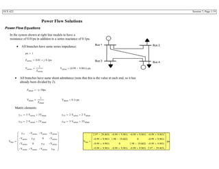
  • 1. ECE 422 Session 7; Page 1/19 Power Flow Solutions Power Flow Equations In the system shown at right line models to have a resistance of 0.01pu in addition to a series reactance of 0.1pu. Bus 1 Bus 3 Bus 2 Bus 4 All branches have same series impedance:  pu 1  Zseries 0.01 j 0.1  pu   Yseries 1 Zseries  Yseries 0.99 9.901i  ( ) pu   All branches have same shunt admittance (note that this is the value at each end, so it has  already been divided by 2). Zshunt j  10  pu  Yshunt 1 Zshunt  Yshunt 0.1i pu   Matrix elements: y11 3 Yseries  3Yshunt   y33 2 Yseries  2 Yshunt    y22 2 Yseries  2Yshunt   y44 3 Yseries  3Yshunt   Ybus y11 Yseries  Yseries  Yseries  Yseries  y22 0 Yseries  Yseries  0 y33 Yseries  Yseries  Yseries  Yseries  y44              Ybus 2.97 29.403i  0.99  9.901i  0.99  9.901i  0.99  9.901i  0.99  9.901i  1.98 19.602i  0 0.99  9.901i  0.99  9.901i  0 1.98 19.602i  0.99  9.901i  0.99  9.901i  0.99  9.901i  0.99  9.901i  2.97 29.403i              pu  
  • 2. ECE 422 Session 7; Page 2/19 Reset origin for matrix and vector subscripts from 0 to 1. ORIGIN 1  Complex Form Equations: S1 V1 V1   Ybus 1 1    V1 V2   Ybus 1 2     V1 V3   Ybus 1 3     V1 V4   Ybus 1 4     = S2 V2 V1   Ybus 2 1    V2 V2   Ybus 2 2     V2 V4   Ybus 2 4     = S3 V3 V1   Ybus 3 1    V3 V3   Ybus 3 3     V3 V4   Ybus 3 4     = S4 V4 V1   Ybus 4 1    V4 V2   Ybus 4 2     V4 V3   Ybus 4 3     V4 V4   Ybus 4 4     = Find real and imaginary parts of the Ybus matrix: G Re Ybus    G 2.97 0.99  0.99  0.99  0.99  1.98 0 0.99  0.99  0 1.98 0.99  0.99  0.99  0.99  2.97              B Im Ybus    B 29.403  9.901 9.901 9.901 9.901 19.602  0 9.901 9.901 0 19.602  9.901 9.901 9.901 9.901 29.403              
  • 3. ECE 422 Session 7; Page 3/19 Rectangular Form P1 V1  2 G 1 1   V1 V2  G 1 2  cos θ1 θ2  ( )  B 1 2  sin θ1 θ2  ( )       V1 V3  G 1 3  cos θ1 θ3  ( )  B 1 3  sin θ1 θ3  ( )       V1 V4  G 1 4  cos θ1 θ4  ( )  B 1 4  sin θ1 θ4  ( )      = P2 V2 V1  G 2 1  cos θ2 θ1  ( )  B 2 1  sin θ2 θ1  ( )      V2  2 G 2 2    V2 V4  G 2 4  cos θ2 θ4  ( )  B 2 4  sin θ2 θ4  ( )       = P3 V3 V1  G 3 1  cos θ3 θ1  ( )  B 3 1  sin θ3 θ1  ( )      V3  2 G 3 3    V3 V4  G 3 4  cos θ3 θ4  ( )  B 3 4  sin θ3 θ4  ( )       = P4 V4 V1  G 4 1  cos θ4 θ1  ( )  B 4 1  sin θ4 θ1  ( )      V4 V2  G 4 2  cos θ4 θ2  ( )  B 4 2  sin θ4 θ2  ( )       V4 V3  G 4 3  cos θ4 θ3  ( )  B 4 3  sin θ4 θ3  ( )       V4  2 G 4   = Q1 V1  2  B 1 1   V1 V2  G 1 2  sin θ1 θ2  ( )  B 1 2  cos θ1 θ2  ( )       V1 V3  G 1 3  sin θ1 θ3  ( )  B 1 3  cos θ1 θ3  ( )       V1 V4  G 1 4  sin θ1 θ4  ( )  B 1 4  cos θ1  (      = Q2 V2 V1  G 2 1  sin θ2 θ1  ( )  B 2 1  cos θ2 θ1  ( )      V2  2 B 2 2    V2 V4  G 2 4  sin θ2 θ4  ( )  B 2 4  cos θ2 θ4  ( )       = Q3 V3 V1  G 3 1  sin θ3 θ1  ( )  B 3 1  cos θ3 θ1  ( )      V3  2 B 3 3    V3 V4  G 3 4  sin θ3 θ4  ( )  B 3 4  cos θ3 θ4  ( )       = Q4 V4 V1  G 4 1  sin θ4 θ1  ( )  B 4 1  cos θ4 θ1  ( )      V4 V2  G 4 2  sin θ4 θ2  ( )  B 4 2  cos θ4 θ2  ( )       V4 V3  G 4 3  sin θ4 θ3  ( )  B 4 3  cos θ4 θ3  ( )       V4  2 B 4   = You could plug the numbers for Gi,j and Bi,j into the equations next.
  • 4. ECE 422 Session 7; Page 4/19 Newton-Raphson Example 1: Reset origin for matrix and vector subscripts from 1 back to 0. ORIGIN 0  Use a simpler Ybus Ybus j  19.98  j 10  j 10  j 10  j  19.98  j 10  j 10  j 10  j  19.98           P2 0.5  P3 1   Q2 0.5  Q3 1   Slack Bus: V1m 1.0  θ1 0  Initial Guesses: V2m0 1.0  θ20 0  V3m0 1.0  θ30 0  Power flow equations using initial guess: P20 V2m0 V1m  Im Ybus 1 0     sin θ20 θ1  ( )  V2m0 V3m0  Im Ybus 1 2     sin θ20 θ30  ( )    P30 V3m0 V1m  Im Ybus 2 0     sin θ30 θ1  ( )  V3m0 V2m0  Im Ybus 2 1     sin θ30 θ20  ( )    Q20 V2m0  V1m  Im Ybus 1 0     cos θ20 θ1  ( )  V2m0 2 Im Ybus 1 1      V2m0 V3m0  Im Ybus 1 2     cos θ20 θ30  ( )    Q30 V3m0  V1m  Im Ybus 2 0     cos θ30 θ1  ( )  V3m0 V2m0  Im Ybus 2 1     cos θ30 θ20  ( )   V3m0 2 Im Ybus 2 2       Initial Mismatch Vector: Use a "1-norm" ΔH0 P2 P20  P3 P30  Q2 Q20  Q3 Q30               ΔH0 0.5 1  0.52 0.98               norm_1 out 0  out out ΔH0 x   x 0 3   for  norm_1 3  well out of tolerance
  • 5. ECE 422 Session 7; Page 5/19 Jacobian Terms J11 submatrix JP2θ2_0 Im Ybus 1 0    V2m0  V1m  cos θ20 θ1  ( )  Im Ybus 1 2    V2m0  V3m0  cos θ20 θ30  ( )    JP2θ3_0 Im Ybus 1 2     V2m0  V3m0  cos θ20 θ30  ( )   JP3θ2_0 Im Ybus 2 1     V3m0  V2m0  cos θ30 θ20  ( )   JP3θ3_0 Im Ybus 2 0    V3m0  V1m  cos θ30 θ1  ( )  Im Ybus 2 1    V3m0  V2m0  cos θ30 θ20  ( )    J12 submatrix JP2Vm2_0 Im Ybus 1 0    V1m  sin θ20 θ1  ( )  Im Ybus 1 2    V3m0  sin θ20 θ30  ( )    JP2Vm3_0 Im Ybus 1 2    V2m0  sin θ20 θ30  ( )   JP3Vm2_0 Im Ybus 2 1    V3m0  sin θ30 θ20  ( )   JP3Vm3_0 Im Ybus 2 0    V1m  sin θ30 θ1  ( )  Im Ybus 2 1    V2m0  sin θ30 θ20  ( )    J21 submatrix JQ2θ2_0 Im Ybus 1 0    V2m0  V1m  sin θ20 θ1  ( )  Im Ybus 1 2    V2m0  V3m0  sin θ20 θ30  ( )    JQ2θ3_0 Im Ybus 1 2     V2m0  V3m0  sin θ20 θ30  ( )   JQ3θ2_0 Im Ybus 2 1     V3m0  V2m0  sin θ30 θ20  ( )   JQ3θ3_0 Im Ybus 2 0    V3m0  V1m  sin θ30 θ1  ( )  Im Ybus 2 1    V3m0  V2m0  sin θ30 θ20  ( )    J22 submatrix JQ2Vm2_0 Im Ybus 1 0     V1m  cos θ20 θ1  ( )  2 V2m0  Im Ybus 1 1      Im Ybus 1 2    V3m0  cos θ20 θ30  ( )    JQ2Vm3_0 Im Ybus 1 2     V2m0  cos θ20 θ30  ( )   JQ3Vm2_0 Im Ybus 2 1     V3m0  cos θ30 θ20  ( )   JQ3Vm3_0 Im Ybus 2 0     V1m  cos θ30 θ1  ( )  Im Ybus 2 1    V2m0  cos θ30 θ20  ( )   2 V3m0  Im Ybus 2 2      
  • 6. ECE 422 Session 7; Page 6/19 J_0 JP2θ2_0 JP3θ2_0 JQ2θ2_0 JQ3θ2_0 JP2θ3_0 JP3θ3_0 JQ2θ3_0 JQ3θ3_0 JP2Vm2_0 JP3Vm2_0 JQ2Vm2_0 JQ3Vm2_0 JP2Vm3_0 JP3Vm3_0 JQ2Vm3_0 JQ3Vm3_0              J_0 20 10  0 0 10  20 0 0 0 0 19.96 10  0 0 10  19.96              Now solve for x (note, I'm using the built-in matrix inverse, but for a large case, one would use LU factorization Δx1 J_0 1  ΔH0   Δx1 0 0.05  1.941 10 3   0.048               θ21 θ20 Δx1 0   θ21 0 deg   θ31 θ30 Δx1 1   θ31 2.865  deg   V2m1 V2m0 Δx1 2   V2m1 1.002  V3m1 V3m0 Δx1 3   V3m1 0.952  Power flow equations using result of iteration 1: P21 V2m1 V1m  Im Ybus 1 0     sin θ21 θ1  ( )  V2m1 V3m1  Im Ybus 1 2     sin θ21 θ31  ( )    P31 V3m1 V1m  Im Ybus 2 0     sin θ31 θ1  ( )  V3m1 V2m1  Im Ybus 2 1     sin θ31 θ21  ( )    Q21 V2m1  V1m  Im Ybus 1 0     cos θ21 θ1  ( )  V2m1 2 Im Ybus 1 1      V2m1 V3m1  Im Ybus 1 2     cos θ21 θ31  ( )    Q31 V3m1  V1m  Im Ybus 2 0     cos θ31 θ1  ( )  V3m1 V2m1  Im Ybus 2 1     cos θ31 θ21  ( )   V3m1 2 Im Ybus 2 2      
  • 7. ECE 422 Session 7; Page 7/19 Updated Mismatch Vector: Use a "1-norm" ΔH1 P2 P21  P3 P31  Q2 Q21  Q3 Q31               ΔH1 0.023 0.048  0.013  0.071               norm_11_NR out 0  out out ΔH1 x   x 0 3   for  good improvement norm_11_NR 0.155  Jacobian Terms J11 submatrix JP2θ2_1 Im Ybus 1 0    V2m1  V1m  cos θ21 θ1  ( )  Im Ybus 1 2    V2m1  V3m1  cos θ21 θ31  ( )    JP2θ3_1 Im Ybus 1 2     V2m1  V3m1  cos θ21 θ31  ( )   JP3θ2_1 Im Ybus 2 1     V3m1  V2m1  cos θ31 θ21  ( )   JP3θ3_1 Im Ybus 2 0    V3m1  V1m  cos θ31 θ1  ( )  Im Ybus 2 1    V3m1  V2m1  cos θ31 θ21  ( )    J12 submatrix JP2Vm2_1 Im Ybus 1 0    V1m  sin θ21 θ1  ( )  Im Ybus 1 2    V3m1  sin θ21 θ31  ( )    JP2Vm3_1 Im Ybus 1 2    V2m1  sin θ21 θ31  ( )   JP3Vm2_1 Im Ybus 2 1    V3m1  sin θ31 θ21  ( )   JP3Vm3_1 Im Ybus 2 0    V1m  sin θ31 θ1  ( )  Im Ybus 2 1    V2m1  sin θ31 θ21  ( )    J21 submatrix JQ2θ2_1 Im Ybus 1 0    V2m1  V1m  sin θ21 θ1  ( )  Im Ybus 1 2    V2m1  V3m1  sin θ21 θ31  ( )    JQ2θ3_1 Im Ybus 1 2     V2m1  V3m1  sin θ21 θ31  ( )   JQ3θ2_1 Im Ybus 2 1     V3m1  V2m1  sin θ31 θ21  ( )   JQ3θ3_1 Im Ybus 2 0    V3m1  V1m  sin θ31 θ1  ( )  Im Ybus 2 1    V3m1  V2m1  sin θ31 θ21  ( )   
  • 8. ECE 422 Session 7; Page 8/19 J22 submatrix JQ2Vm2_1 Im Ybus 1 0     V1m  cos θ21 θ1  ( )  2 V2m1  Im Ybus 1 1      Im Ybus 1 2    V3m1  cos θ21 θ31  ( )    JQ2Vm3_1 Im Ybus 1 2     V2m1  cos θ21 θ31  ( )   JQ3Vm2_1 Im Ybus 2 1     V3m1  cos θ31 θ21  ( )   JQ3Vm3_1 Im Ybus 2 0     V1m  cos θ31 θ1  ( )  Im Ybus 2 1    V2m1  cos θ31 θ21  ( )   2 V3m1  Im Ybus 2 2       J_1 JP2θ2_1 JP3θ2_1 JQ2θ2_1 JQ3θ2_1 JP2θ3_1 JP3θ3_1 JQ2θ3_1 JQ3θ3_1 JP2Vm2_1 JP3Vm2_1 JQ2Vm2_1 JQ3Vm2_1 JP2Vm3_1 JP3Vm3_1 JQ2Vm3_1 JQ3Vm3_1              J_1 19.545 9.525  0.477 0.477 9.525  19.032 0.477  0.952  0.476 0.476  20.531 9.507  0.501 1.001  10.007  18.043              Now solve for x Δx2 J_1 1  ΔH1   Δx2 2.542 10 5   2.894  10 3   3.621  10 3   5.998  10 3                    θ22 θ21 Δx2 0   θ22 1.457 10 3   deg   θ32 θ31 Δx2 1   θ32 3.031  deg   V2m2 V2m1 Δx2 2   V2m2 0.998  V3m2 V3m1 Δx2 3   V3m2 0.946 
  • 9. ECE 422 Session 7; Page 9/19 Power flow equations using result of iteration 2: P22 V2m2 V1m  Im Ybus 1 0     sin θ22 θ1  ( )  V2m2 V3m2  Im Ybus 1 2     sin θ22 θ32  ( )    P32 V3m2 V1m  Im Ybus 2 0     sin θ32 θ1  ( )  V3m2 V2m2  Im Ybus 2 1     sin θ32 θ22  ( )    Q22 V2m2  V1m  Im Ybus 1 0     cos θ22 θ1  ( )  V2m2 2 Im Ybus 1 1      V2m2 V3m2  Im Ybus 1 2     cos θ22 θ32  ( )    Q32 V3m2  V1m  Im Ybus 2 0     cos θ32 θ1  ( )  V3m2 V2m2  Im Ybus 2 1     cos θ32 θ22  ( )   V3m2 2 Im Ybus 2 2       Updated Mismatch Vector: Use a "1-norm" ΔH2 P2 P22  P3 P32  Q2 Q22  Q3 Q32               ΔH2 2.672 10 4   4.417  10 4   7.148  10 5   5.592  10 4                    norm_12_FD out 0  out out ΔH2 x   x 0 3   for  norm_12_FD 1.34 10 3    close to a desirable tolerance Find P and Q at slack bus: P1 V1m V2m2  Im Ybus 0 1     sin θ1 θ22  ( )  V1m V3m2  Im Ybus 0 2     sin θ1 θ32  ( )    P1 0.5  P1 P2  1  Q1 V1m 2  Im Ybus 0 0     V2m2 Im Ybus 0 1     cos θ1 θ22  ( )   V1m V3m2  Im Ybus 0 2     cos θ1 θ32  ( )    Q1 0.551  Q1 Q22  1.051 
  • 10. ECE 422 Session 7; Page 10/19 Newton-Raphson Example 2: Now suppose that we were given that the voltage at bus 2 is know (voltage regulated bus): V2m 1.02  Now V2m is no longer an unknown, which reduces the size of the problem to solve Power flow equations using initial guess: P20 V2m V1m  Im Ybus 1 0     sin θ20 θ1  ( )  V2m V3m0  Im Ybus 1 2     sin θ20 θ30  ( )    P30 V3m0 V1m  Im Ybus 2 0     sin θ30 θ1  ( )  V3m0 V2m  Im Ybus 2 1     sin θ30 θ20  ( )    Q2 equation is no longer needed here Q30 V3m0  V1m  Im Ybus 2 0     cos θ30 θ1  ( )  V3m0 V2m  Im Ybus 2 1     cos θ30 θ20  ( )   V3m0 2 Im Ybus 2 2       Initial Mismatch Vector: Use a "1-norm" ΔH0 P2 P20  P3 P30  Q3 Q30           ΔH0 0.5 1  0.78           norm_1 out 0  out out ΔH0 x   x 0 2   for  norm_1 2.28  well out of tolerance Jacobian Terms J11 submatrix JP2θ2_0 Im Ybus 1 0    V2m  V1m  cos θ20 θ1  ( )  Im Ybus 1 2    V2m  V3m0  cos θ20 θ30  ( )    JP2θ3_0 Im Ybus 1 2     V2m  V3m0  cos θ20 θ30  ( )   JP3θ2_0 Im Ybus 2 1     V3m0  V2m  cos θ30 θ20  ( )   JP3θ3_0 Im Ybus 2 0    V3m0  V1m  cos θ30 θ1  ( )  Im Ybus 2 1    V3m0  V2m  cos θ30 θ20  ( )   
  • 11. ECE 422 Session 7; Page 11/19 J12 submatrix (no longer have partials with respect to V2m) JP2Vm3_0 Im Ybus 1 2    V2m  sin θ20 θ30  ( )   JP3Vm3_0 Im Ybus 2 0    V1m  sin θ30 θ1  ( )  Im Ybus 2 1    V2m  sin θ30 θ20  ( )    J21 submatrix (no longer have Q2 terms) JQ3θ2_0 Im Ybus 2 1     V3m0  V2m  sin θ30 θ20  ( )   JQ3θ3_0 Im Ybus 2 0    V3m0  V1m  sin θ30 θ1  ( )  Im Ybus 2 1    V3m0  V2m  sin θ30 θ20  ( )    J22 submatrix JQ2Vm3_0 Im Ybus 1 2     V2m  cos θ20 θ30  ( )   JQ3Vm3_0 Im Ybus 2 0     V1m  cos θ30 θ1  ( )  Im Ybus 2 1    V2m  cos θ30 θ20  ( )   2 V3m0  Im Ybus 2 2       J_0 JP2θ2_0 JP3θ2_0 JQ3θ2_0 JP2θ3_0 JP3θ3_0 JQ3θ3_0 JP2Vm3_0 JP3Vm3_0 JQ3Vm3_0          J_0 20.4 10.2  0 10.2  20.2 0 0 0 19.76          Now solve for x (note, I'm using the built-in matrix inverse, but for a large case, we would use LU factorization Δx1 J_0 1  ΔH0   Δx1 3.246  10 4   0.05  0.039             θ21 θ20 Δx1 0   θ21 0.019  deg   θ31 θ30 Δx1 1   θ31 2.846  deg   V3m1 V3m0 Δx1 2   V3m1 0.961 
  • 12. ECE 422 Session 7; Page 12/19 Power flow equations using result of iteration 1: P21 V2m V1m  Im Ybus 1 0     sin θ21 θ1  ( )  V2m V3m1  Im Ybus 1 2     sin θ21 θ31  ( )    P31 V3m1 V1m  Im Ybus 2 0     sin θ31 θ1  ( )  V3m1 V2m  Im Ybus 2 1     sin θ31 θ21  ( )    Q31 V3m1  V1m  Im Ybus 2 0     cos θ31 θ1  ( )  V3m1 V2m  Im Ybus 2 1     cos θ31 θ21  ( )   V3m1 2 Im Ybus 2 2       Updated Mismatch Vector: Use a "1-norm" ΔH1 P2 P21  P3 P31  Q3 Q31           ΔH1 0.02 0.04  0.055           norm_1 out 0  out out ΔH1 x   x 0 2   for  norm_1 0.115  Jacobian Terms J11 submatrix JP2θ2_1 Im Ybus 1 0    V2m  V1m  cos θ21 θ1  ( )  Im Ybus 1 2    V2m  V3m1  cos θ21 θ31  ( )    JP2θ3_1 Im Ybus 1 2     V2m  V3m1  cos θ21 θ31  ( )   JP3θ2_1 Im Ybus 2 1     V3m1  V2m  cos θ31 θ21  ( )   JP3θ3_1 Im Ybus 2 0    V3m1  V1m  cos θ31 θ1  ( )  Im Ybus 2 1    V3m1  V2m  cos θ31 θ21  ( )    J12 submatrix JP2Vm3_1 Im Ybus 1 2    V2m  sin θ21 θ31  ( )   JP3Vm3_1 Im Ybus 2 0    V1m  sin θ31 θ1  ( )  Im Ybus 2 1    V2m  sin θ31 θ21  ( )    J21 submatrix JQ3θ2_1 Im Ybus 2 1     V3m1  V2m  sin θ31 θ21  ( )   JQ3θ3_1 Im Ybus 2 0    V3m1  V1m  sin θ31 θ1  ( )  Im Ybus 2 1    V3m1  V2m  sin θ31 θ21  ( )    J22 submatrix JQ3Vm3_1 Im Ybus 2 0     V1m  cos θ31 θ1  ( )  Im Ybus 2 1    V2m  cos θ31 θ21  ( )   2 V3m1  Im Ybus 2 2      
  • 13. ECE 422 Session 7; Page 13/19 J_1 JP2θ2_1 JP3θ2_1 JQ3θ2_1 JP2θ3_1 JP3θ3_1 JQ3θ3_1 JP2Vm3_1 JP3Vm3_1 JQ3Vm3_1          J_1 19.985 9.785  0.483 9.785  19.379 0.96  0.503 1  18.207          Now solve for x (note, I'm using the built-in matrix inverse, but for a large case, we would use LU factorization Δx2 J_1 1  ΔH1   Δx2 4.782  10 6   2.221  10 3   3.132  10 3                θ22 θ21 Δx2 0   θ22 0.019  deg   θ32 θ31 Δx2 1   θ32 2.973  deg   V3m2 V3m1 Δx2 2   V3m2 0.957  Power flow equations using result of iteration 2: P22 V2m V1m  Im Ybus 1 0     sin θ22 θ1  ( )  V2m V3m2  Im Ybus 1 2     sin θ22 θ32  ( )    P32 V3m2 V1m  Im Ybus 2 0     sin θ32 θ1  ( )  V3m2 V2m  Im Ybus 2 1     sin θ32 θ22  ( )    Q32 V3m2  V1m  Im Ybus 2 0     cos θ32 θ1  ( )  V3m2 V2m  Im Ybus 2 1     cos θ32 θ22  ( )   V3m2 2 Im Ybus 2 2       Updated Mismatch Vector: Use a "1-norm" ΔH2 P2 P22  P3 P32  Q3 Q32           ΔH2 7.193 10 5   1.426  10 4   2.366  10 4                norm_1 out 0  out out ΔH2 x   x 0 2   for  norm_1 4.512 10 4    close to a desirable tolerance
  • 14. ECE 422 Session 7; Page 14/19 Find P and Q at slack bus: P1 V1m V2m2  Im Ybus 0 1     sin θ1 θ22  ( )  V1m V3m2  Im Ybus 0 2     sin θ1 θ32  ( )    P1 0.5  P1 P2  1  Q1 V1m 2  Im Ybus 0 0     V2m2 Im Ybus 0 1     cos θ1 θ22  ( )   V1m V3m2  Im Ybus 0 2     cos θ1 θ32  ( )    Q1 0.436  and now find Q2 Q2 V2m  V1m  Im Ybus 1 0     cos θ22 θ1  ( )  V2m 2 Im Ybus 1 1      V2m V3m2  Im Ybus 1 2     cos θ22 θ32  ( )    Q2 0.835  Repeat Using Fast Decoupled Load Flow for Example 1 Start from the same initial guesses, the same power flow equations and the same mismatch vector as the first example above.  Initial Mismatch Vector: Use a "1-norm" ΔH0 P2 P20  P3 P30  Q2 Q20  Q3 Q30               ΔH0 0.5 1  0.855 0.78               norm_1 out 0  out out ΔH0 x   x 0 3   for  norm_1 3.135  Well out of toleranec Or using the 2-norm norm_2sq out 0  out out ΔH0 x   2   x 0 3   for  norm_2 norm_2sq  norm_2 1.609  well out of tolerance
  • 15. ECE 422 Session 7; Page 15/19 Or we could also evaluate using the infinity norm: norm_infinity max ΔH0      norm_infinity 1  Fast Decoupled Load Flow Set Up 1: B1 for the P equations (imaginary part of Ybus with slack bus row/column 1 removed): B1 Im submatrix Ybus 1  2  1  2  ( ) ( )  B1 19.98  10 10 19.98         B2 for Q equations (same dimension, since the same number of unknown voltages and unknown angles) B2 Im submatrix Ybus 1  2  1  2  ( ) ( )  B2 19.98  10 10 19.98         Now modify mismatch vector by dividing by voltage magnitudes.... ΔH0mod P2 P20  ( ) V2m0 P3 P30  ( ) V3m0 Q2 Q20  ( ) V2m0 Q3 Q30  ( ) V3m0                        ΔH0mod 0.5 1  0.855 0.78               Now break the mismatch into P and Q equations ΔP0 submatrix ΔH0mod 0  1  0  0  ( )  ΔP0 0.5 1        
  • 16. ECE 422 Session 7; Page 16/19 ΔQ0 submatrix ΔH0mod 2  3  0  0  ( )  ΔQ0 0.855 0.78         Δθ1 B1 1   ΔP0   Δθ1 1.915  10 3   2.8686        deg  ΔVm1 B2 1   ΔQ0   ΔVm1 0.031 0.0235         θ21 θ20 Δθ1 0   θ21 1.915  10 3   deg  θ31 θ30 Δθ1 1   θ31 2.869  deg  V2m1 V2m0 ΔVm1 0   V2m1 1.031  V3m1 V3m0 ΔVm1 1   V3m1 0.976  Power flow equations using result of iteration 1: P21 V2m1 V1m  Im Ybus 1 0     sin θ21 θ1  ( )  V2m1 V3m1  Im Ybus 1 2     sin θ21 θ31  ( )    P31 V3m1 V1m  Im Ybus 2 0     sin θ31 θ1  ( )  V3m1 V2m1  Im Ybus 2 1     sin θ31 θ21  ( )    Q21 V2m1  V1m  Im Ybus 1 0     cos θ21 θ1  ( )  V2m1 2 Im Ybus 1 1      V2m1 V3m1  Im Ybus 1 2     cos θ21 θ31  ( )    Q31 V3m1  V1m  Im Ybus 2 0     cos θ31 θ1  ( )  V3m1 V2m1  Im Ybus 2 1     cos θ31 θ21  ( )   V3m1 2 Im Ybus 2 2      
  • 17. ECE 422 Session 7; Page 17/19 Updated Mismatch Vector: Use a "1-norm" ΔH1fd P2 P21  P3 P31  Q2 Q21  Q3 Q31               ΔH1fd 3.162  10 3   7.805  10 3   0.038  0.244                 norm_11_fd out 0  out out ΔH1fd x   x 0 3   for  norm_11_fd 0.293  good improvement For comparison, after 1 iteration on the same system Newton-Raphson had: norm_11_NR 0.155  Faster improvement Now do a second iteration  ΔH1modfd P2 P21  ( ) V2m1 P3 P31  ( ) V3m1 Q2 Q21  ( ) V2m1 Q3 Q31  ( ) V3m1                        ΔH1modfd 3.066  10 3   7.993  10 3   0.037  0.25                 Now break the mismatch into P and Q equations ΔP1 submatrix ΔH1modfd 0  1  0  0     ΔP1 3.066  10 3   7.993  10 3            ΔQ1 submatrix ΔH1modfd 2  3  0  0     ΔQ1 0.037  0.25        
  • 18. ECE 422 Session 7; Page 18/19 Δθ2 B1 1   ΔP1   Δθ2 0.027  0.0365        deg  ΔVm2 B2 1   ΔQ1   ΔVm2 0.0108  0.0179         θ22 θ21 Δθ2 0   θ22 0.029  deg  θ32 θ31 Δθ2 1   θ32 2.905  deg  V2m2 V2m0 ΔVm1 0   V2m2 1.031  V3m2 V3m0 ΔVm1 1   V3m2 0.976  Power flow equations using result of iteration 2: P22 V2m2 V1m  Im Ybus 1 0     sin θ22 θ1  ( )  V2m2 V3m2  Im Ybus 1 2     sin θ22 θ32  ( )    P32 V3m2 V1m  Im Ybus 2 0     sin θ32 θ1  ( )  V3m2 V2m2  Im Ybus 2 1     sin θ32 θ22  ( )    Q22 V2m2  V1m  Im Ybus 1 0     cos θ22 θ1  ( )  V2m2 2 Im Ybus 1 1      V2m2 V3m2  Im Ybus 1 2     cos θ22 θ32  ( )    Q32 V3m2  V1m  Im Ybus 2 0     cos θ32 θ1  ( )  V3m2 V2m2  Im Ybus 2 1     cos θ32 θ22  ( )   V3m2 2 Im Ybus 2 2       Updated Mismatch Vector: Use a "1-norm" ΔH2fd P2 P22  P3 P32  Q2 Q22  Q3 Q32               ΔH2fd 5.166 10 5   5.223 10 5   0.039  0.244                 norm_12_fd out 0  out out ΔH2fd x   x 0 3   for  norm_12_fd 0.283  close to a desirable tolerance
  • 19. ECE 422 Session 7; Page 19/19 Compare to after iteration 1: norm_11_fd 0.293  Notice that we have a small change Compare to after iteration 2 of Newton Raphson: norm_12_FD 1.34 10 3    Much faster progress, but more computational intense.