Download to read offline

![MATLAB CODE :
clear all
close all
clc
annee=2020;
switch annee
case 2020
load profil_ve_20
load temps_arrive_1200
load Nb_etat_tr
load Nb_etat_dom
vei=round(profil_ve(1:52560,1)/3.7);
M_vei=zeros(144,365);
for i=1:365
M_vei(:,i)=vei(144*(i-1)+1:144*i);
if sum(M_vei(:,i))<sum(Nb_etat_tr+Nb_etat_dom)
M_vei(:,i)=round(M_vei(:,i)*(sum(Nb_etat_tr+Nb_etat_dom)/sum(M_vei(:,i))));
end
end
nb_ve=1200;
case 2030
load Nb_etat_tr_30
load Nb_etat_dom_30
load profil_ve_30
load temps_arrive_1200
vei=round(profil_ve(1:52560,1)/3.7);
M_vei=zeros(144,365);
for i=1:365
M_vei(:,i)=vei(144*(i-1)+1:144*i);
if sum(M_vei(:,i))<sum(Nb_etat_tr+Nb_etat_dom)
M_vei(:,i)=round(M_vei(:,i)*(sum(Nb_etat_tr+Nb_etat_dom)/sum(M_vei(:,i))));
end
end
nb_ve=1200
end
Tve=[];
Pr_nw=[];
ref= []; % jours
Be=[];
A=[];
B=[];
ordre=[];
VE=[];
for m=1:2
m
Y_tr =zeros(nb_ve,144);
Y_dom =zeros(nb_ve,144);](https://image.slidesharecdn.com/b3c55414-240d-4f0c-9f7c-18077aa14969-150407142152-conversion-gate01/75/L2EP_report-6-2048.jpg)
![Nb_etat_dom_i= zeros(nb_ve,1);
Nb_etat_tr_i= zeros(nb_ve,1);
vei_tr=M_vei(1:66,m);
vei_dom=M_vei(67:144,m);
if sum(vei_tr)<sum(Nb_etat_tr)
vei_tr=round(vei_tr*(sum(Nb_etat_tr)/sum(vei_tr))+0.5);
end
if sum(vei_dom)<sum(Nb_etat_dom)
vei_dom=round(vei_dom*(sum(Nb_etat_dom)/sum(vei_dom))+0.5);
end
ve_rep=[vei_tr ; vei_dom ];
g=[vei_tr ; vei_dom ];
ref= [ref;g] ;
limit_tr=66;
limit_dom=144;
or = zeros (nb_ve,1);
a= zeros (143,1);
BEd=(Nb_etat_tr+Nb_etat_dom);
%***********************Chargement_travail*********************************
[bs_tr, b_tr] = sort(Nb_etat_tr,'descend');
for j=1:66
j;
for k=1:nb_ve
i=b_tr(k);
if sum(Y_tr(i,:))<Nb_etat_tr(i,1) && debut_tr(i)<=j
if ve_rep(j)>0
ve_rep(j)= ve_rep(j)-1;
Y_tr(i,j)=1;
else if Nb_etat_tr(i)- ((limit_tr-j)+sum(Y_tr(i,:)))>0
ve_rep(j)= ve_rep(j)-1;
Y_tr(i,j)=1;
else
Y_tr(i,j)=0;
end
end
end
end
end
%************************Chargement_domicile*******************************
[bs_dom, b_dom] = sort(Nb_etat_dom,'descend');
for j=67:144
j;
for k=1:nb_ve
c=0;
i=b_dom(k);](https://image.slidesharecdn.com/b3c55414-240d-4f0c-9f7c-18077aa14969-150407142152-conversion-gate01/75/L2EP_report-7-2048.jpg)
![if sum(Y_dom(i,:))<Nb_etat_dom(i,1) && debut_dom(i)<=j
if ve_rep(j)>0
ve_rep(j)= ve_rep(j)-1;
Y_dom(i,j)=1;
else if Nb_etat_dom(i)- ((limit_dom-j)+sum(Y_dom(i,:)))>0
ve_rep(j)= ve_rep(j)-1;
Y_dom(i,j)=1;
else
Y_dom(i,j)=0;
end
end
end
end
end
%**************************ORDRES******************************************
Ytotale = Y_tr+Y_dom;
c=0;
for i=1:nb_ve
for j=1:143
a(j)=Ytotale(i,j+1)-Ytotale(i,j);
if a(j)~=0
c=c+1;
end
end
or(i)=c;
c=0;
end
%**************************VE**********************************************
VEc=0;
BEr=(sum(Ytotale'))';
dif= BEd-BEr;
for i=1:nb_ve
if dif(i)~= 0
VEc=VEc+1;
end
end
VE =[VE VEc];
ordre= [ordre or];
Pr_nw=[ Pr_nw sum(Y_tr+Y_dom) ];
A = [A (sum(Y_tr'))' ];
B = [B (sum(Y_dom'))'];
end
Pr=sum(Pr_nw) ;
Be=[Be A+B ];
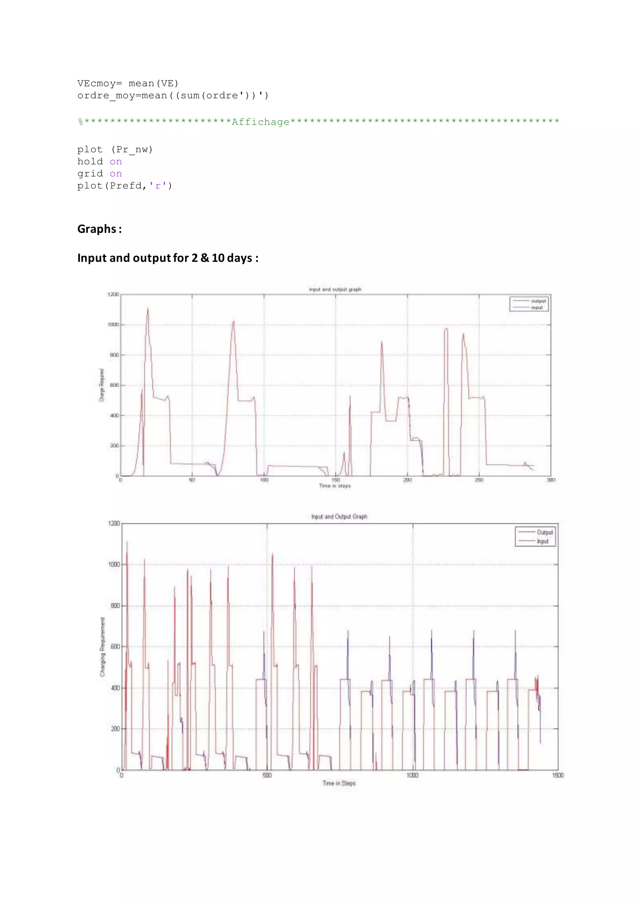
Prefd=ref';
%***********************Indicateurs****************************************
err_ve=100*(((Pr)-sum(Prefd))/sum(Prefd))
err_final = 100*((sum(Pr) - sum(Prefd))/sum(Prefd))
err_BE=100*((sum(sum( Be))-
m*sum(Nb_etat_tr+Nb_etat_dom))/(m*sum(Nb_etat_tr+Nb_etat_dom)))](https://image.slidesharecdn.com/b3c55414-240d-4f0c-9f7c-18077aa14969-150407142152-conversion-gate01/75/L2EP_report-8-2048.jpg)
![MATLAB CODE FOR THE DELAY :
%%%%%%%% Chargement retard %%%%%%%%%%%%%%%%%%%%%%%%%%%%%%%%%%%%%%%%%%%%%%%%
retard_tr = zeros(1200,2);
retard_dom = zeros(1200,2);
for i = 1:1200
for j = 1:66
l = i;
if Y_tr(i,j) == 1
retard_tr(l,1) = j;
break;
end
end
end
for i = 1:1200
for j = 67:144
l = i;
if Y_dom(i,j) == 1
retard_dom(l,1) = j;
break;
end
end
end
taille =1200;
if taille>=1
for l = 1:taille
retard_tr(l,2) = 6 ;
retard_dom(l,2) = 6 ;
end
for l = taille+1:1200
retard_tr(l,2) = 0;
retard_dom(l,2) = 0;
end
Yfinal_tr = Y_tr;
Yfinal_dom = Y_dom;
for l = 1:taille
i = b_tr(l);
j = retard_tr(l,1);
Yfinal_tr(i,j:end) = circshift(Yfinal_tr(i,j:end),[0 retard_tr(l,2)]);
for j = retard_tr(l,1):retard_tr(l,1)+retard_tr(l,2)-1
Yfinal_tr(i,j) = 0;
end
end
for l = 1:taille
i = b_dom(l);
j = retard_dom(l,1);
Yfinal_dom(i,j:end) = circshift(Yfinal_dom(i,j:end),[0 retard_dom(l,2)]);
for j = retard_dom(l,1):retard_dom(l,1)+retard_dom(l,2)-1](https://image.slidesharecdn.com/b3c55414-240d-4f0c-9f7c-18077aa14969-150407142152-conversion-gate01/75/L2EP_report-11-2048.jpg)
![Yfinal_dom(i,j) = 0;
end
end
end
Ytotale = Y_tr+Y_dom;
for j=1:1200
for k=67:144
if Yfinal_tr(j,k)==1;
Yfinal_tr(j,k)=0;
end
end
end
Yfinal = Yfinal_tr(:,1:144)+Yfinal_dom(:,1:144);
for i =1:1200
not_char_work(i,1)=sum(Yfinal(i,1:144));
req_work(i,1)=sum(Ytotale(i,1:144));
end
final_work{m} = sum(req_work) - sum(not_char_work);
ve_delay_work{m} = sum(Yfinal(:,1:144));
dif=zeros (1200,1);
T=0;
BEr=(sum(Ytotale'))';
BEfinal=(sum(Yfinal'))';
dif=BEr-BEfinal;
for i=1:1200
if dif(i)~= 0
T=T+1;
end
end
Tve=[Tve T];
final_last_work = cell2mat(final_work);
ve_delay_last_work = cell2mat(ve_delay_work);
veh_not_char_work{m} = nnz(final_last_work(:,m));
data_1 = cell2mat(veh_not_char_work);
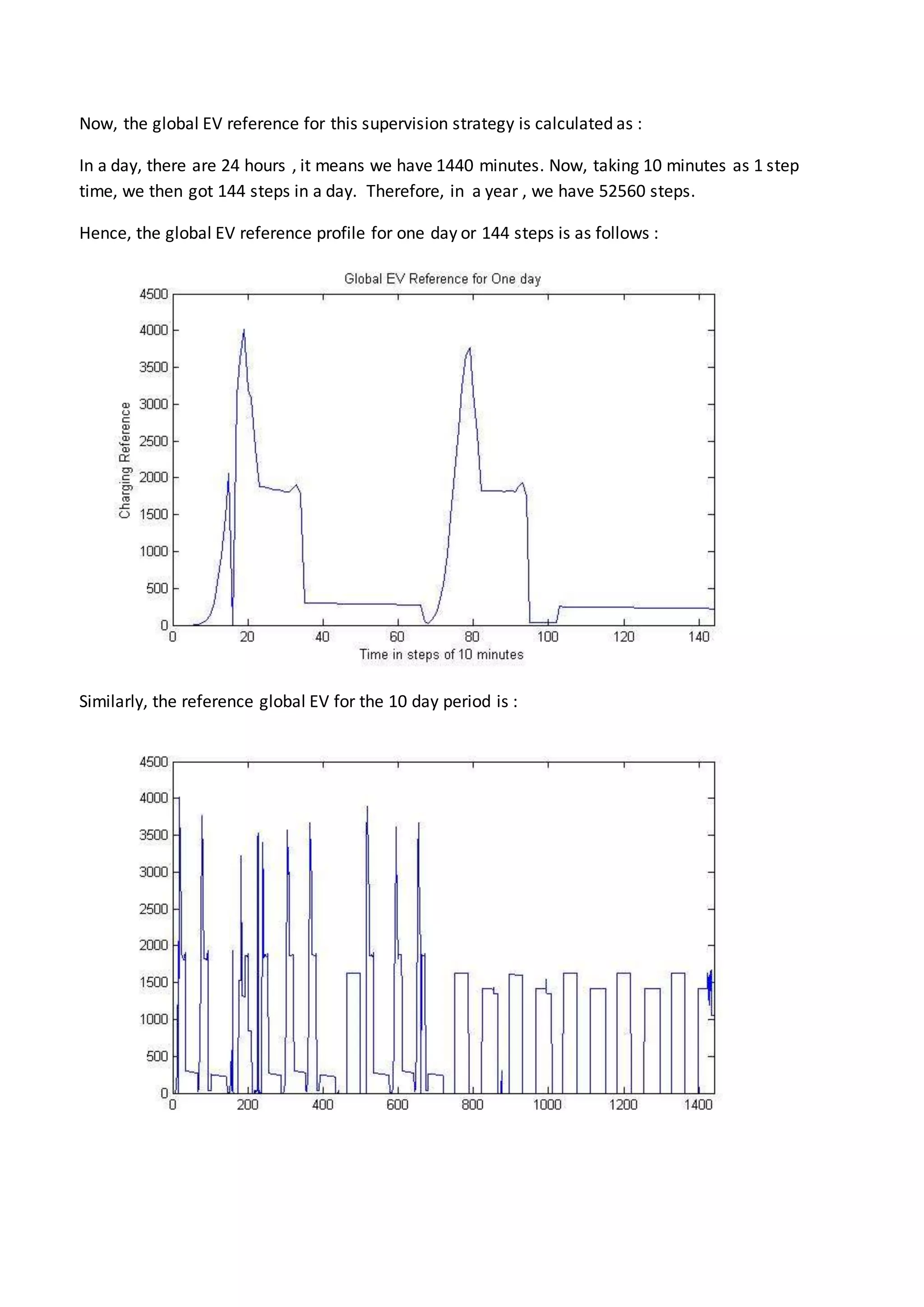
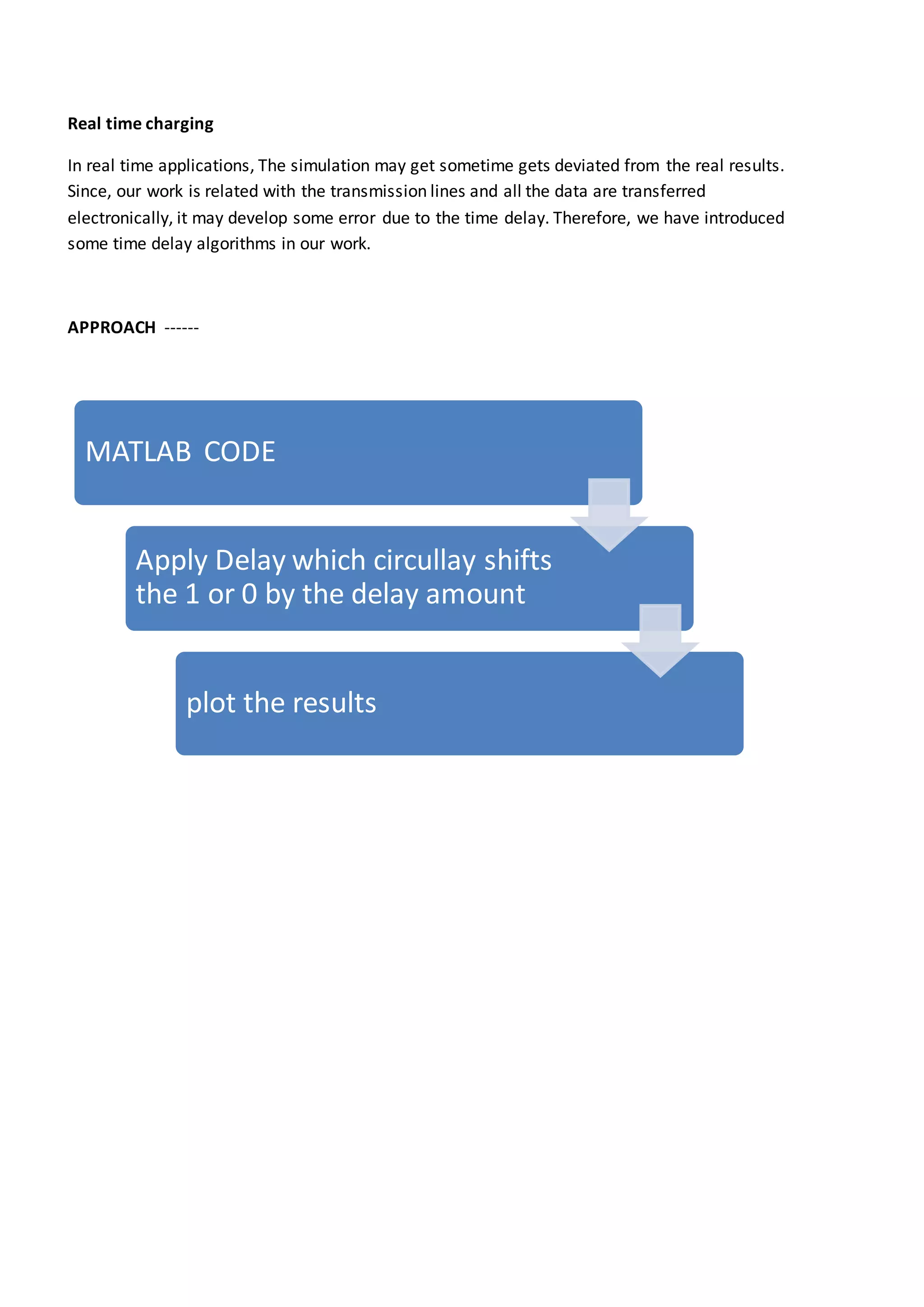
The above code is concatenated with the above previous matlab code to get the full code
with the delay to get the idea of the real analysis of the data transmitted through the full
process.
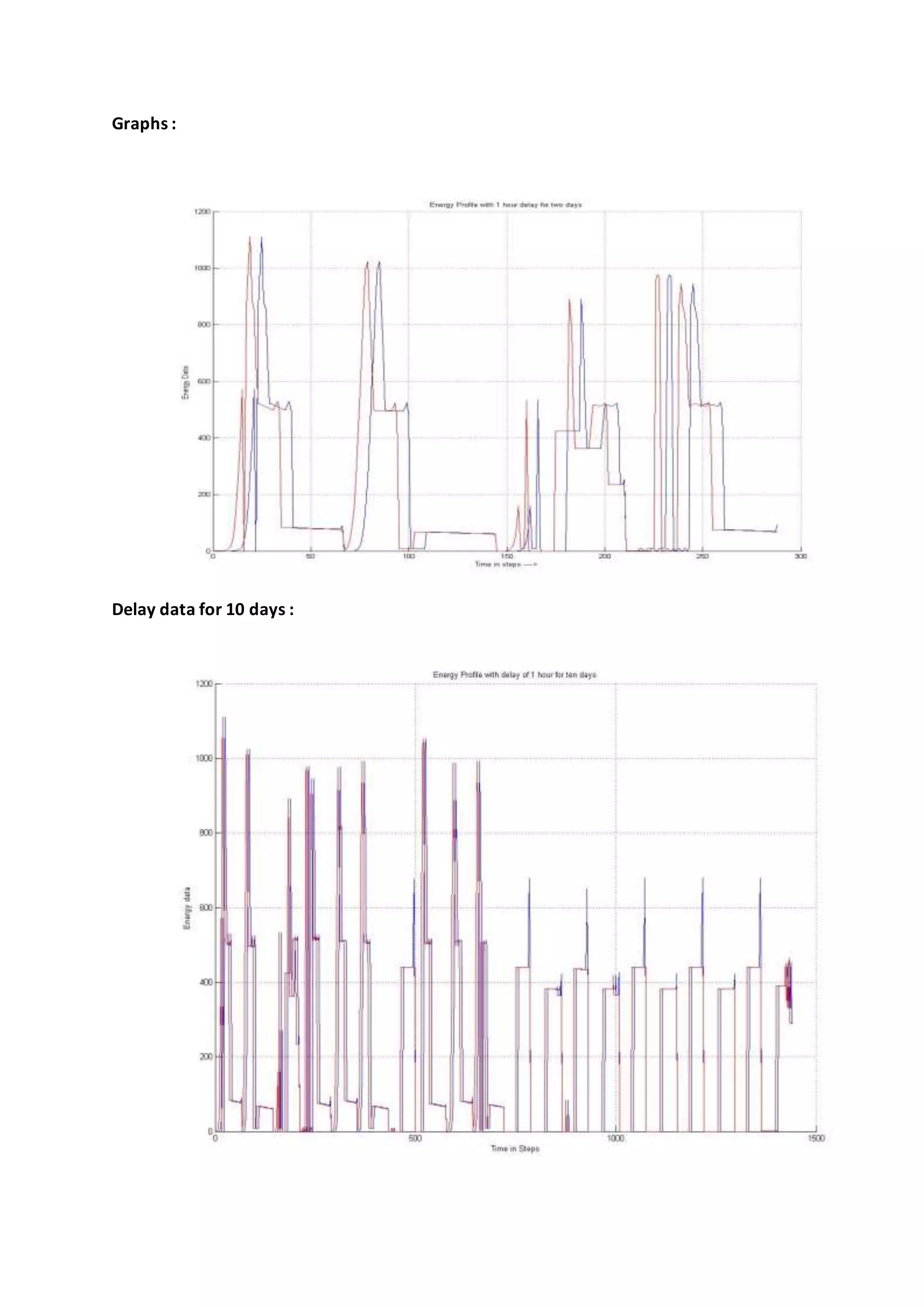
The delay is applied for the two and ten days and the graph is plotted and the number of
vehicles which are not charged are collected.](https://image.slidesharecdn.com/b3c55414-240d-4f0c-9f7c-18077aa14969-150407142152-conversion-gate01/75/L2EP_report-12-2048.jpg)
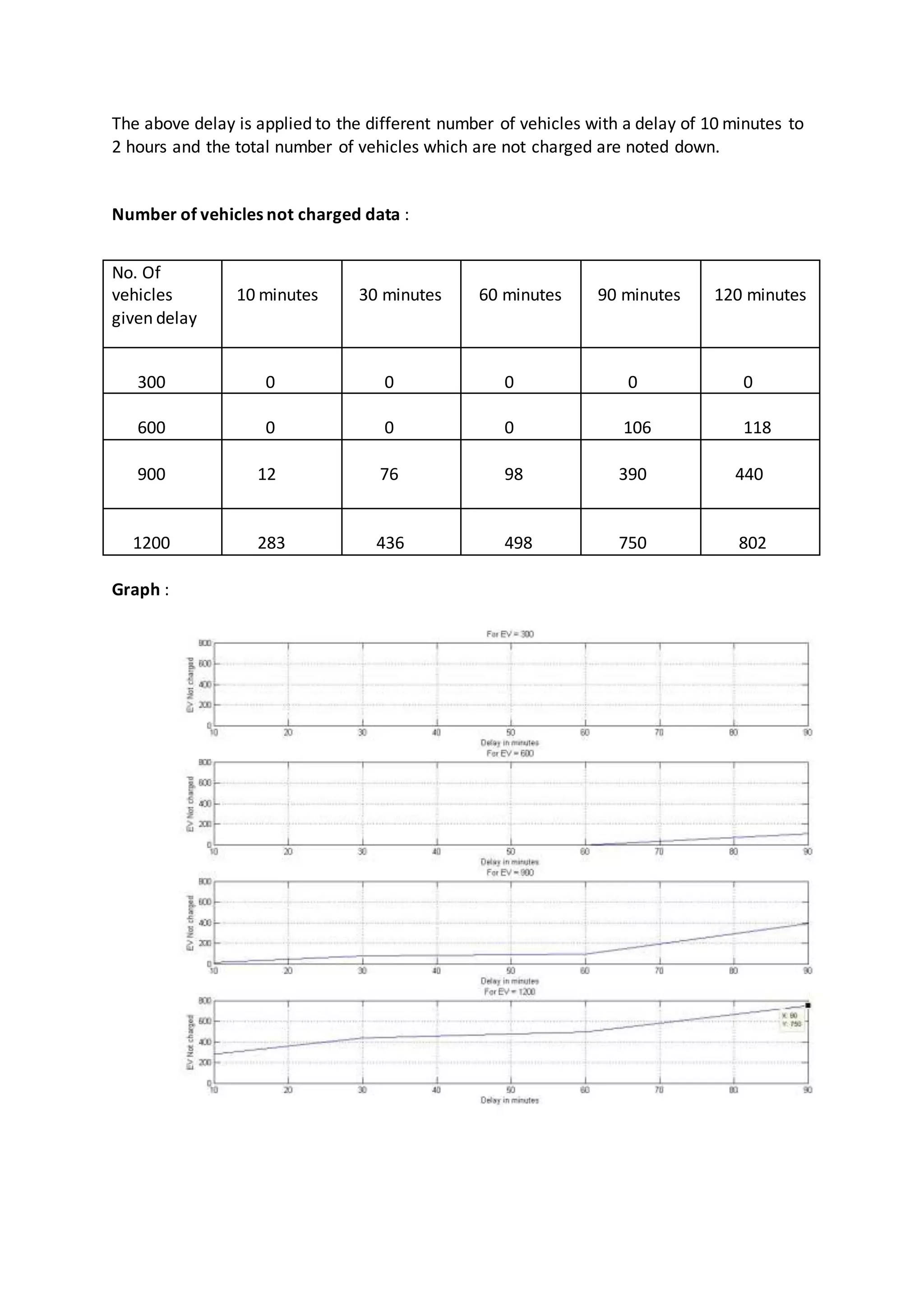

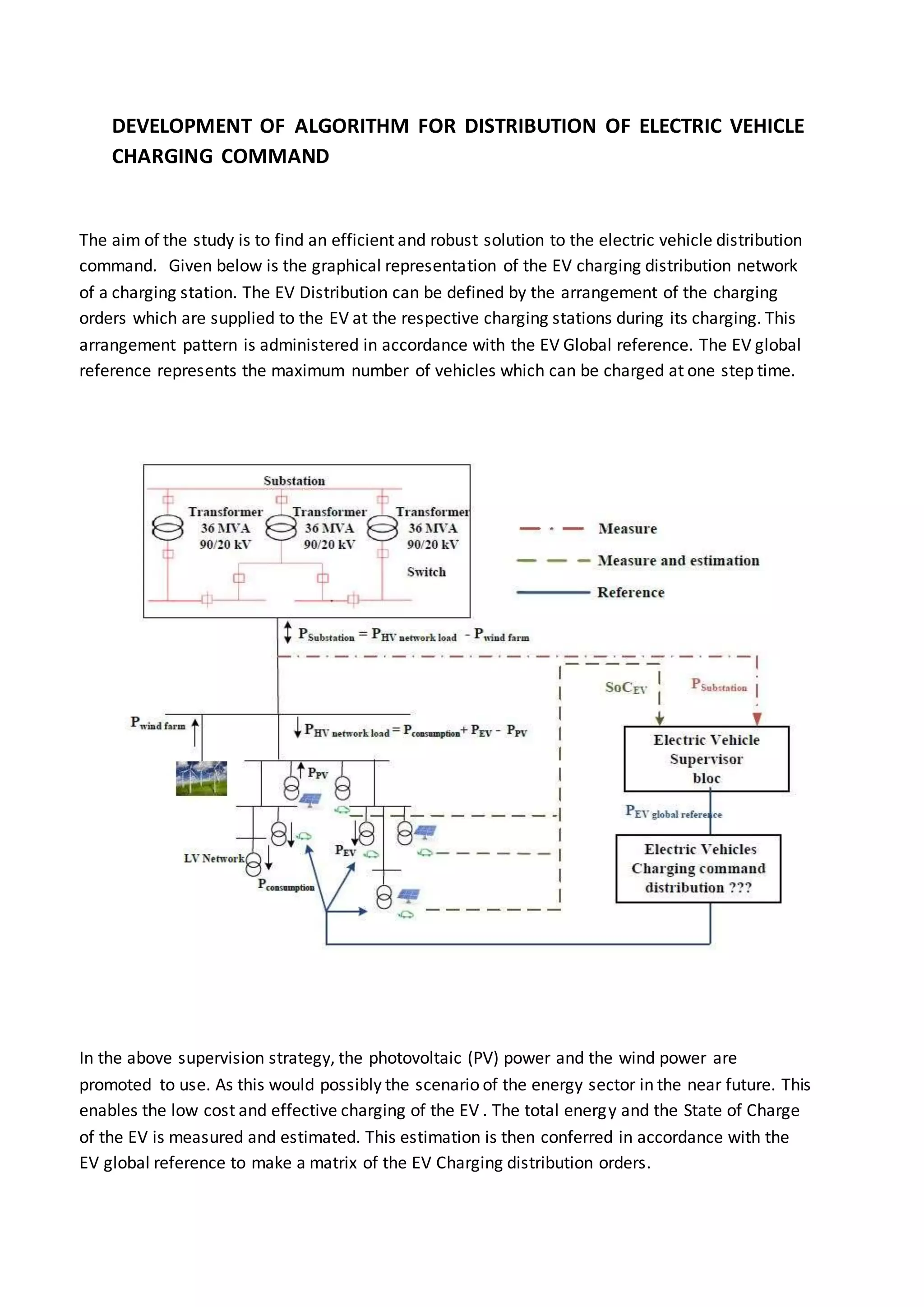
This document summarizes a student's research internship developing an algorithm for distributing electric vehicle charging commands. The aim is to find an efficient solution for scheduling EV charging at stations. The algorithm considers factors like solar and wind power availability, total energy needs, and state of charge for each EV. MATLAB code is used to simulate charging 1200 EVs over days and years, accounting for home and work charging profiles. Effects of transmission delays are also modeled by introducing time shifts to the charging schedules. Results show higher delays lead to more EVs not receiving full charges.


