Kush Defense

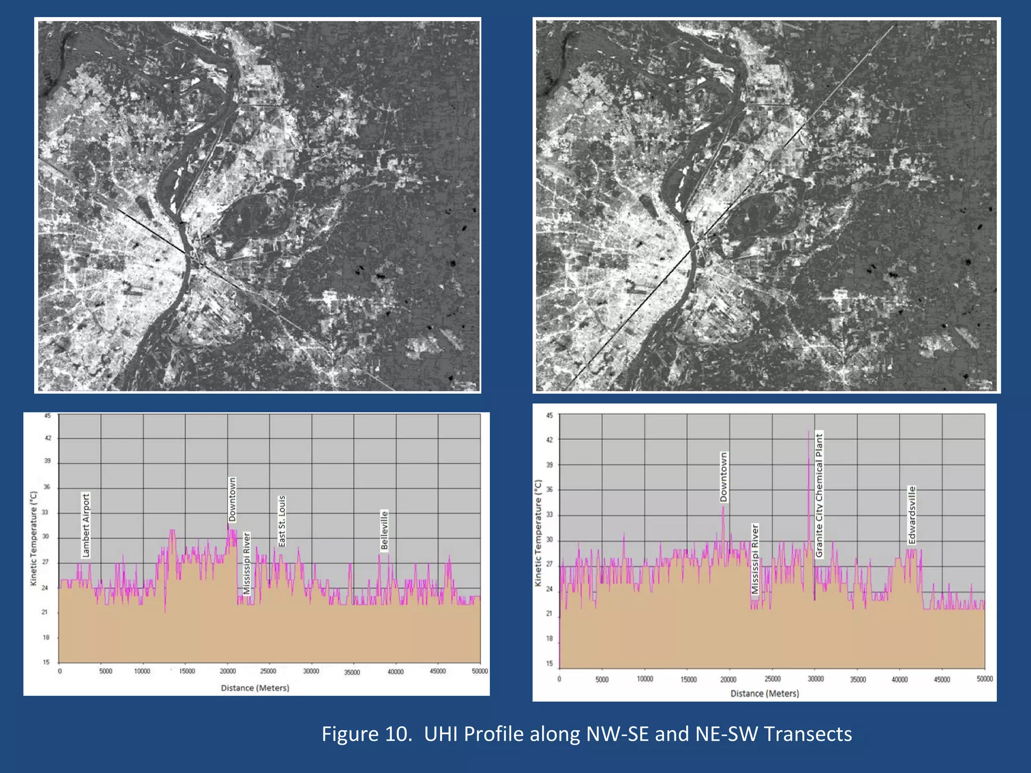
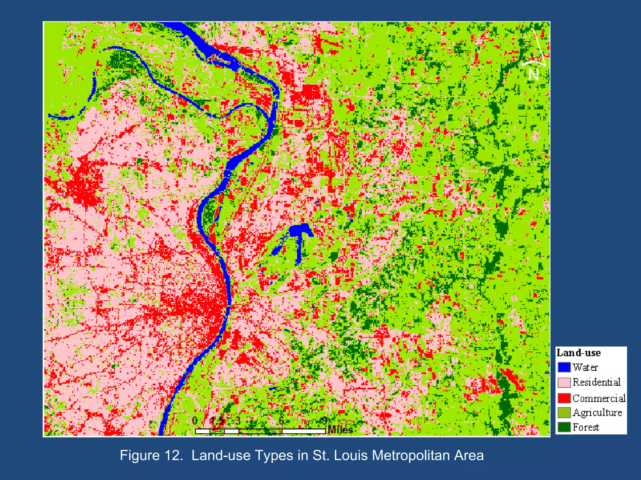
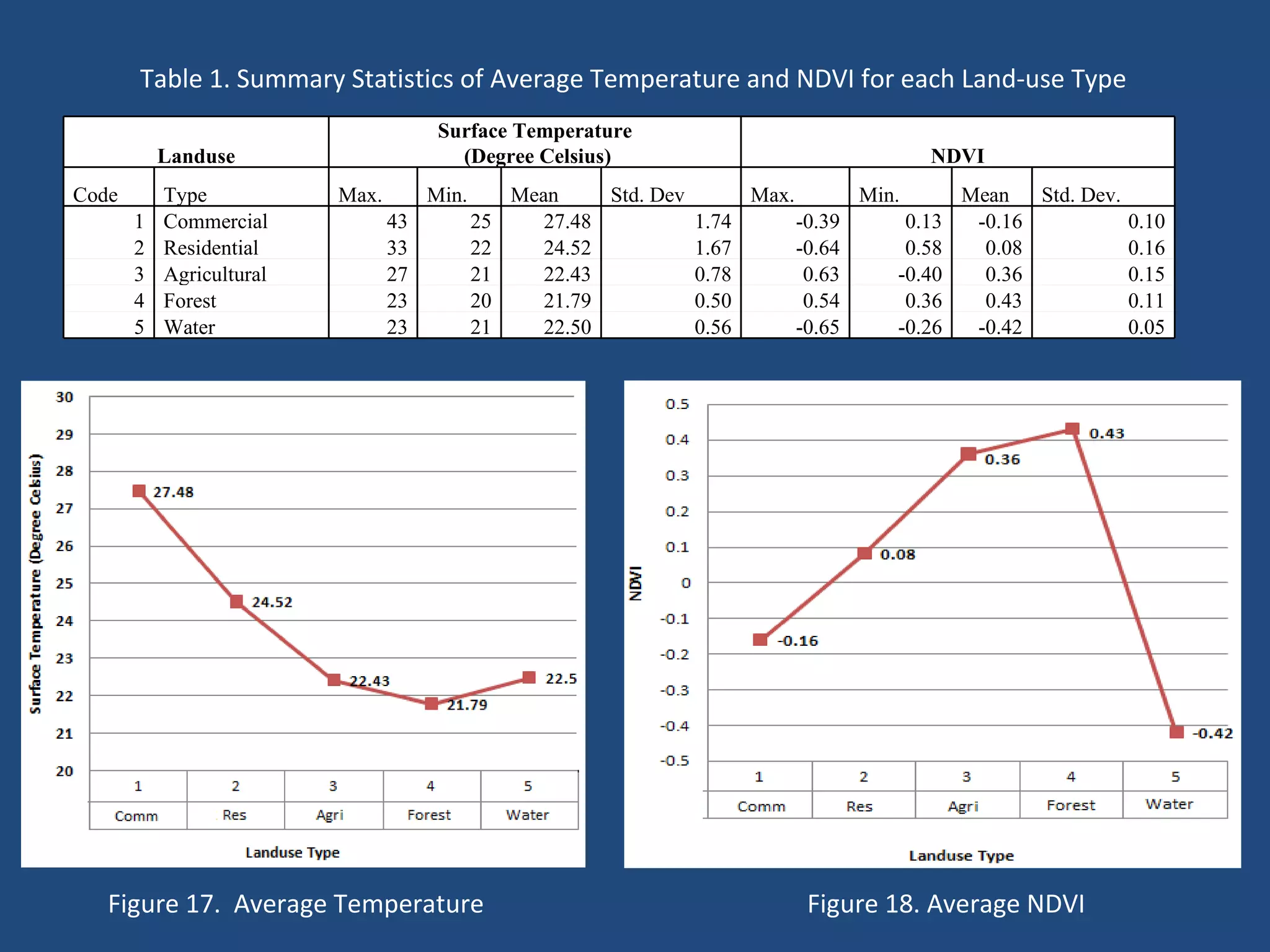
A Remote Sensing Study of the Urban Heat Island (UHI) Effect in the St. Louis Metropolitan Area, MO Kusumakar Bhusal

Introduction Literature Review Objectives Research Questions Methodology Results Discussions & Conclusions Recommendations References

Introduction Urban Heat Island (UHI) : Noticeable difference in temperature profile between the City and its outskirts Elevated air and surface temperatures in urban areas relative to surrounding suburban and rural areas (Solecki et al. 2005) Figure 1. Classic UHI Pattern in a City Area (Source – EPA 2006 )

Figure 2. The Urban Energy Budget Source: EPA 2006 SUN

Literature Review Spatial variation of the UHI can be determined by the analysis of multi temporal remote sensing images (Chen et al 2006) Identifying the land surface temperature is a key aspect while studying the UHI phenomenon in remote sensing studies. Land surface temperature can be estimated by satellite thermal infrared sensors with different spatial resolution (Li et al 2004) Over the past decades, high resolution satellite data have been used in studying the UHI distribution patterns in cities such as Atlanta, Houston, Indianapolis & New York

Very limited studies in identifying the UHI pattern of St. Louis region using satellite remote sensing technique Clark and Peterson (1972) discussed that the heat island intensity within St. Louis varied with structural density index which was based upon the population density, commercial and industrial land-use at that time Matson et al (1978) compared the surface temperature difference for the City and the rural areas with the help of Advanced Very High Resolution Radiometer (AVHRR) thermal sensor with 0.9 km resolution

Even though high resolution satellite imageries have been used to characterize the UHI effect in many US Cities, St. Louis has been fairly untouched area in recent past Gap in literature The need for the study is even more pronounced as the City is expanding and growing in terms of population and economy Present study using the latest remote sensing technique is of high significance in delineating the UHI pattern of the St. Louis metropolitan area

Objectives To determine the spatial distribution of the UHI in St. Louis metropolitan area using Landsat 7 Enhanced Thematic Mapper (ETM+) satellite data To examine the relationship between Land surface temperature, Normalized Difference Vegetation Index (NDVI) and land-use Patterns

Research Questions What is the spatial pattern of the UHI in the St. Louis metropolitan area? How the UHI is influenced by surface temperature variation and vegetation abundance? How does the land-use affect spatial distribution of the UHI? Is there a significant difference in average surface temperature between different land-use types?

Methodology Study Area Metropolitan St. Louis Figure 3. Landsat ETM+ Satellite Capture

Data Resources Landsat 7 ETM+ Band 6 thermal image Band width (10.4 – 12.5 micrometer) Spatial Resolution 60m Date: 28 th July 2002, SLC on Mode Path 023, Row 033 - Satellite Overpass Time - 4:20 GMT (10:20 am central time) Projection : UTM zone 14, Datum : WGS 84 Georeferenced to UTM coordinate system Figure 5. Landsat 7 Satellite

- May 31, 2003, the Scan Line Corrector (SLC), which compensates for the forward motion of Landsat 7 failed. - Without an operating SLC, ETM+ line traces a zigzag pattern along the satellite ground track which leaves gap in image - This error is still not fixed in Landsat satellite

Image Analysis Step 1: Conversion of Image Digital Numbers to Radiance: - Digital Numbers (DN) of band 6 converted to radiance and then the effective at satellite temperature - Eventually, the radiant temperature image was converted to Kinetic Image to reflect the land surface temperature

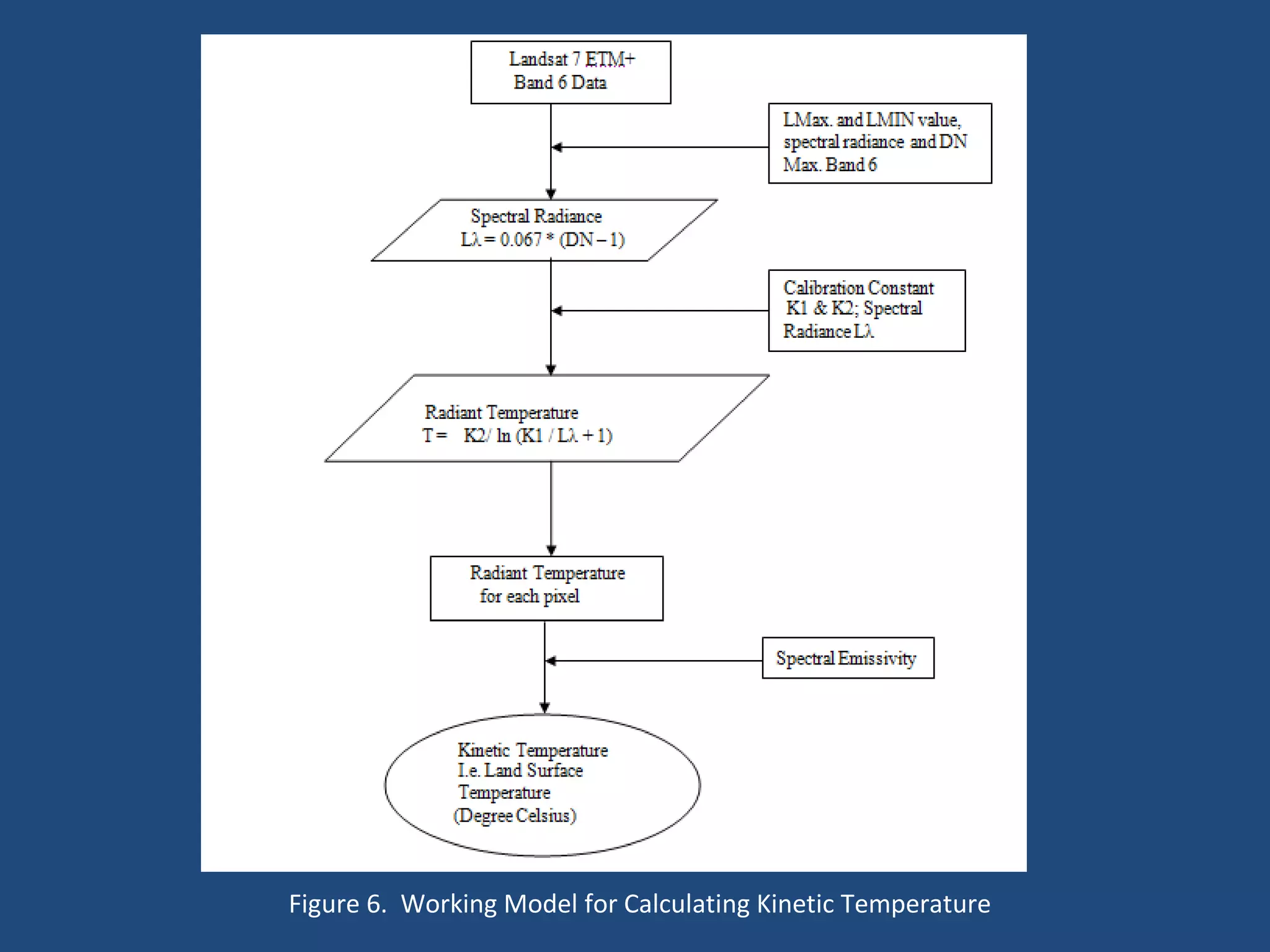
Radiance (Lλ) = (LMAX λ – LMIN λ / QCALMAX – QCALMIN) * (QCAL – QCALMIN) + LMIN λ (Source – Landsat users manual, 2000 )…………………………………………………[1] Where, Lλ = Spectral radiance at sensor’s aperture in (watts / meter sq.*ster*μm) QCAL = Quantized Calibrated pixel value in Digital Numbers (DN) LMIN λ & LMAX λ = Spectral Radiance for Band 6 at DN 1 and 255 respectively. LMIN λ = 0; LMaxλ = 17.040 QCALMIN = minimum quantized calibrated pixel value corresponding to LMIN in DN i.e. DN Min= 1 QCALMAX = maximum quantized calibrated pixel value corresponding to LMIN in DN i.e. DN Max= 255

Step 2: Conversion from Radiance to Radiant Temperature: Tb = {K2 / ln (K1 / Lλ + 1)} ……………………………..[2] ( Source: Chen et al 2006 ) Where, Tb = Radiant temperature K1 = Calibration constant 1 = 666.09 K2 = Calibration constant 2 = 1282.71 Lλ = Spectral radiance in watts / meter sq.*ster*micrometer

Step 3: Conversion to Kinetic Temperature: St = {Tb / (1 + (λ + Tb/ ρ)*lnε)} ……………………………[3] (Source: Weng et al 2006) Where, St = Surface kinetic Temperature Tb = Radiant Temperature λ = wavelength (μm) ρ = h*c/σ = 1.438*10 -2 (m K) σ = Boltzmann constant (1.38*10 -23 J/K) h = Planck’s constant (6.626*10 -34 Js) c = velocity of light (2.998*10 8 m/s) ε = emissivity constant

Average emissivity values for common surface materials were used. The emissivity classification was referred from Lilesand and Kiefer (2007) Table 1. Typical Emissivities of Common materials Over the range of 8 – 14 µm Material Average Emissivity (µm) Clear water 0.98 – 0.99 Wet Snow 0.98 – 0.99 Green Vegetation 0.96 – 0.99 Asphaltic concrete 0.95 – 0.98 Glass 0.77 – 0.81 Aluminum foil 0.03 – 0.07 Highly polished gold 0.02 – 0.03

Figure 6. Working Model for Calculating Kinetic Temperature

Surface temperature map was generated by running the model Spatial temperature profile was created across different transects on the image Altogether 4 transects were constructed that ran in different directions across the study area Transects were constructed in such a manner that they all covered major land-use within the study area and intersected at a common point in main City center

Figure 7. Transect Overlay on Surface Temperature Map

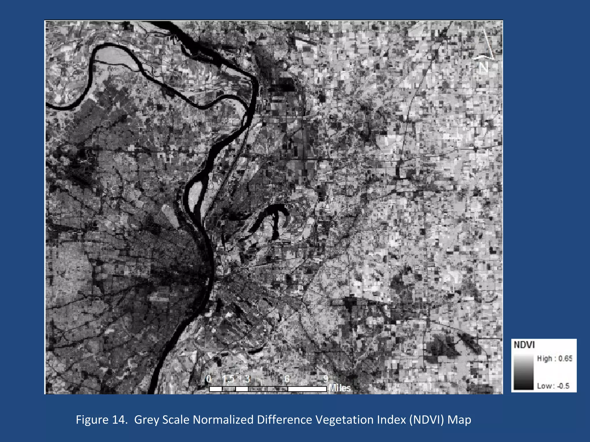
Normalized Difference Vegetation Index (NDVI) Calculation: NDVI - used to express the vegetation density. Considered to be a good indicator of surface temperature while studying the UHI phenomenon (Weng 2001). NDVI image created from visible red (0.63 -0.69μm) and near infrared (NIR) (0.76 – 0.90μm) bands NIR – Red NDVI = NIR + Red ………………………….[4]

Land-use Classification: Physical characterization of the land cover Classified using supervised classification technique with the maximum likelihood algorithm Involved 3 different stages : Training stage - Representative training sets were defined based on the spectral attributes Classification stage - Pixels were categorized into land use classes it closely resembled Output - Classified land-use map

Correlation Analysis: Statistical correlation established between land surface temperature, NDVI and Land use land cover. Pearson’s correlation was run with significance level 0.01 Software used - SPSS Version 16

Test of Significance To determine if there was significant difference in average temperature based on land-use types Pair wise t test conducted to examine the difference between mean temperature in each land-use type Each land-use type was treated as an independent sample. Hypothesis tested to analyze if one mean is significantly higher or lower than the other for different land-use combination

Null Hypothesis (Ho): The mean surface temperature in commercial land-use is not significantly greater from that of the residential land-use. Alternative Hypothesis (Ha): The mean surface temperature in commercial land-use is significantly greater than that of residential land-use (Similar hypothesis created for other different combination of land-uses) Level of Significance (α) = 0.01

Table. Land-use Combinations used Commercial / Residential Commercial / Agricultural Commercial / Forest Commercial / water Residential / Agricultural Residential / Forest Residential / Water Agricultural / Forest Agricultural / Water Forest / Water

Test Statistic (t) = (M1 – M2 / Sd) Where, M1 = Mean surface temperature for Commercial land-use M2 = Mean surface temperature for Residential land-use Sd = standard error

Since two different samples were analyzed in each pair with different mean and standard deviation, pooled standard deviation was used in order to achieve the improved estimate of the standard error. Sp = √ S1² / n1 + S2² / n2 Where, Sp = Standard error with pooled standard deviation S1 & S2 = Standard deviation for land-use classes with n1 and n2 sample sizes respectively n1 & n2 = Sample size

Figure 8. Land Surface Temperature (Grey Scale ) Results

Figure 9. UHI Profile along WE and NS Transects

Figure 10. UHI Profile along NW-SE and NE-SW Transects

Figure 11. Spatial Distribution of UHI in St. Louis Area

Figure 12. Land-use Types in St. Louis Metropolitan Area

Figure 13. Land-use Map - 3D View

Figure 14. Grey Scale Normalized Difference Vegetation Index (NDVI) Map

Figure 15. Classified Normalized Difference Vegetation Index (NDVI) Map

Figure 16. Comparison between Surface Temperature, Land-use and NDVI

Figure 17. Average Temperature Figure 18. Average NDVI Table 1. Summary Statistics of Average Temperature and NDVI for each Land-use Type Landuse Surface Temperature (Degree Celsius) NDVI Code Type Max. Min. Mean Std. Dev Max. Min. Mean Std. Dev. 1 Commercial 43 25 27.48 1.74 -0.39 0.13 -0.16 0.10 2 Residential 33 22 24.52 1.67 -0.64 0.58 0.08 0.16 3 Agricultural 27 21 22.43 0.78 0.63 -0.40 0.36 0.15 4 Forest 23 20 21.79 0.50 0.54 0.36 0.43 0.11 5 Water 23 21 22.50 0.56 -0.65 -0.26 -0.42 0.05

Comparison of Means Table 2. Pairwise t- test Comparison One tailed t-test Land-use Combination t-score Sig. Level ( α) Comm. / Res. 485.2 0.01 Comm. / Agri. 1578 0.01 Comm. / Forest 1016.07 0.01 Comm. / Water 1310.52 0.01 Res. / Agri 267.94 0.01 Res. / Forest 557.1 0.01 Res. / Water 748.14 0.01 Agri. / Forest 193.93 0.01 Agri. / Water 8.75 0.01 Forest / Water 142 0.01

Calculated t -value largely exceeded the critical value and was way over in the rejection region for each case That is the mean surface temperature in commercial land-use is significantly higher from that of the residential land-use and so on for other combinations The null hypothesis was rejected

Table 3. Correlation Between NDVI and Surface Temperature Correlation Analysis Negative Correlation existed between NDVI and land surface Temperature for all land-use types Land-use Land-use Correlation code Type Coefficient (r) 1 Commercial -0.56 2 Residential -0.30 3 Agricultural -0.25 4 Forest -0.50 5 Water -0.15

Research Questions (Revisited) What is the spatial pattern of the UHI in the St. Louis metropolitan area? Highest temperature zones concentrated in the downtown or the commercial area of the City of St. Louis. Decrease in temperature profile more evident further away from the main city to suburban and rural setting High temperature peaks observed in other smaller Cities and suburban areas away from downtown such as Alton, Granite City, Collinsville, Edwardsville, East St. Louis and Belleville

How the UHI is influenced by surface temperature variation and vegetation abundance? Negative correlation between surface temperature and NDVI revealed that the areas with lower vegetation abundance recorded increase in surface temperature and vice versa. Intensity of the UHI more pronounced in areas with lower vegetation density

How does the land-use affect spatial distribution of the UHI? Average surface temperature was higher in commercial and residential land-use which was characterized by low vegetation abundance (negative NDVI). Lower average was recorded in agricultural and forest land-use where the vegetation abundance was very high (positive NDVI) Is there a significant difference in average surface temperature between different land-use types? The null hypothesis was rejected. Significant difference observed in average surface temperature for built up (residential and commercial) and non built-up land-use (agriculture, forest and water).

Spatial distribution of the UHI in St. Louis metropolitan area was determined using Landsat 7 Enhanced Thematic Mapper (ETM+) satellite data Presence of the UHI effect in St. Louis metropolitan area Elevated temperature profile basically due to more built-up areas and impervious surfaces which absorb and store high amounts of solar radiation Similar to the big City areas, smaller urban or suburban settings can also produce noticeable thermal effects when compared with surrounding rural environment Discussions and Conclusions

Existence of negative correlation between land surface temperature and vegetation abundance. That is higher the surface temperature, lower is the vegetation density and vice versa. NDVI – a good indicator for surface temperature variation. UHI intensity more pronounced in commercial and residential land-use (areas with lower vegetation density) Average surface temperature significantly higher in built-up land-use when compared to non built-up land-use.

Study Limitations Unavailability of up-to-date satellite image Surface measurements taken using remotely sensed images do not always match up with the real world scenario Varying satellite azimuth angle and different thermal properties of horizontal and vertical surfaces might affect the radiance measurement Other factors such as the landscape characteristics, surface roughness, surface emissivity and atmospheric effects can affect the precise measurement of the UHI

Recommendations Planting more trees, shrubs and vegetation in side walks and available open spaces would reduce the UHI effect in the City areas through increased evapotranspiration Using reflective building materials help reflect back the incoming solar radiation rather than absorbing it Green roof option – rooftop gardens and other living vegetations help reduce the surface temperatures

References Finished upon request

Kush Defense

More Related Content

What's hot

Viewers also liked

Similar to Kush Defense

Recently uploaded

Kush Defense

Editor's Notes