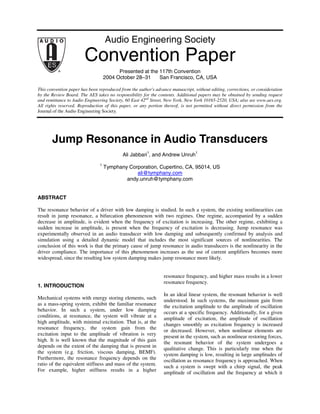
This document is a convention paper that analyzes the phenomenon of "jump resonance" in audio transducers. Jump resonance occurs when a transducer with low damping is driven near its resonance frequency, resulting in sudden increases or decreases in oscillation amplitude depending on the direction of frequency sweep. The paper presents an experimental observation of jump resonance and develops a detailed nonlinear model of a transducer's mechanics and electronics to simulate this behavior. It identifies the primary cause of jump resonance as the nonlinearity in the driver's compliance.

1. Audio Engineering Society
Convention Paper
Presented at the 117th Convention
2004 October 28–31 San Francisco, CA, USA
This convention paper has been reproduced from the author's advance manuscript, without editing, corrections, or consideration
by the Review Board. The AES takes no responsibility for the contents. Additional papers may be obtained by sending request
and remittance to Audio Engineering Society, 60 East 42nd
Street, New York, New York 10165-2520, USA; also see www.aes.org.
All rights reserved. Reproduction of this paper, or any portion thereof, is not permitted without direct permission from the
Journal of the Audio Engineering Society.
Jump Resonance in Audio Transducers
Ali Jabbari1
, and Andrew Unruh1
1
Tymphany Corporation, Cupertino, CA, 95014, US
ali@tymphany.com
andy.unruh@tymphany.com
ABSTRACT
The resonance behavior of a driver with low damping is studied. In such a system, the existing nonlinearities can
result in jump resonance, a bifurcation phenomenon with two regimes. One regime, accompanied by a sudden
decrease in amplitude, is evident when the frequency of excitation is increasing. The other regime, exhibiting a
sudden increase in amplitude, is present when the frequency of excitation is decreasing. Jump resonance was
experimentally observed in an audio transducer with low damping and subsequently confirmed by analysis and
simulation using a detailed dynamic model that includes the most significant sources of nonlinearities. The
conclusion of this work is that the primary cause of jump resonance in audio transducers is the nonlinearity in the
driver compliance. The importance of this phenomenon increases as the use of current amplifiers becomes more
widespread, since the resulting low system damping makes jump resonance more likely.
1. INTRODUCTION
Mechanical systems with energy storing elements, such
as a mass-spring system, exhibit the familiar resonance
behavior. In such a system, under low damping
conditions, at resonance, the system will vibrate at a
high amplitude, with minimal excitation. That is, at the
resonance frequency, the system gain from the
excitation input to the amplitude of vibration is very
high. It is well known that the magnitude of this gain
depends on the extent of the damping that is present in
the system (e.g. friction, viscous damping, BEMF).
Furthermore, the resonance frequency depends on the
ratio of the equivalent stiffness and mass of the system.
For example, higher stiffness results in a higher
resonance frequency, and higher mass results in a lower
resonance frequency.
In an ideal linear system, the resonant behavior is well
understood. In such systems, the maximum gain from
the excitation amplitude to the amplitude of oscillation
occurs at a specific frequency. Additionally, for a given
amplitude of excitation, the amplitude of oscillation
changes smoothly as excitation frequency is increased
or decreased. However, when nonlinear elements are
present in the system, such as nonlinear restoring forces,
the resonant behavior of the system undergoes a
qualitative change. This is particularly true when the
system damping is low, resulting in large amplitudes of
oscillation as resonance frequency is approached. When
such a system is swept with a chirp signal, the peak
amplitude of oscillation and the frequency at which it

2. JABBARI, UNRUH JUMP RESONANCE IN AUDIO TRANSDUCERS
AES 117th Convention, San Francisco, CA, USA, 2004 October 28–31
Page 2 of 10
occurs depend on the direction – increasing or
decreasing frequency – of the chirp signal.
A typical electromagnetic driver, used in most audio
transducers, behaves much like a mass-spring system.
This is particularly true at frequencies well below the
cone breakup frequencies. There are however many
nonlinear elements in such drivers. The most significant
of those are the nonlinearities in the restoring force, the
BL factor, and the inductance. Given that these
nonlinearities are functions of driver cone displacement,
the transducer behaves linearly for small excursions. As
the cone excursion increases, the effects of
nonlinearities become more prominent, resulting in
harmonic and intermodulation distortion. Furthermore,
when the driver damping is low, these nonlinearities
significantly change the resonant behavior of the driver.
The motivation for the analysis, presented in this paper,
is the experimental observation of sudden jumps in the
amplitude of driver excursion near its resonance
frequency. This is manifested as either a sudden
decrease or a sudden increase in the amplitude of
oscillation, depending on the direction from which the
resonance frequency is approached. When the resonance
frequency is approached from a higher frequency there
is a sudden increase in the amplitude of oscillation. On
the other hand, when the resonance frequency is
approached from a lower frequency, there is a sudden
decrease in the amplitude of oscillation. Furthermore,
the frequencies at which these jumps in the amplitude of
cone excursion occur are distinct, which is
representative of a bifurcation phenomenon. In a typical
driver, due to the stiffening nature of the restoring force,
the jump to higher amplitude of oscillation occurs at a
lower frequency than the frequency at which the jump
to lower amplitude of oscillation occurs.
A detailed dynamic model of a typical audio transducer
is developed in order to investigate the observed jump
resonance behavior. The model includes the more
significant nonlinearities present in a typical driver,
namely the nonlinearities in the BL factor, inductance,
and compliance. The resulting dynamic model is used to
determine which of the aforementioned nonlinearities
significantly contribute to the onset of the jump
resonance behavior. Furthermore, with this model, the
effect of varying these nonlinearities and the resulting
effect on the jump phenomenon can be studied.
An analytical treatment of the jump resonance
phenomenon is given for both the undamped and
damped forced oscillation. The effect of softening and
hardening spring, as well as that of increasing system
damping is presented.
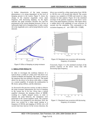
2. NONLINEAR MODEL OF A DRIVER
To investigate the effects of various nonlinearities on
the behavior of a typical driver, a nonlinear model of
such a driver was created. The model is implemented in
Matlab and its graphical interface, Simulink [5,6]. There
are two main components in the model, namely, the
mechanical and the electrical subsystems. Each
subsystem includes the appropriate nonlinear elements
and the governing differential equations. In each
subsystem the various internal states of the system, and
significant parameters and quantities such as forces,
voltages, inductance, BL-factor and others can be
monitored. The two subsystems are interconnected to
each other, as shown in Figure 1.
Figure 1: Mechanical and Electrical Subsystems
The mechanical subsystem models the driver as a point
mass, with a single degree of freedom in x , attached to
a nonlinear spring, and a linear mechanical damper. The
electromagnetic force applied to the point mass is
determined by the current output of the electric block
and the value of the nonlinear BL factor, see equation 1.
ixBLF ⋅= )( (1)

3. JABBARI, UNRUH JUMP RESONANCE IN AUDIO TRANSDUCERS
AES 117th Convention, San Francisco, CA, USA, 2004 October 28–31
Page 3 of 10
It is assumed that the BL factor can be represented as a
nonlinear function of the position of the point mass.
i
n
i
i xbxBL ∑=
=
0
)( (2)
Figure 2: BL curve for a typical driver
Figure 3: Compliance curve for a typical driver
The nonlinear spring force is given by:
xxKFsp ⋅= )( (3)
where )(xK is the nonlinear spring stiffness. Similar to
the BL factor, the spring stiffness can be represented by
a polynomial,
∑∑ ==
==
n
i
i
i
n
i
i
i
xc
xkxK
00
1
)( (4)
where
i
n
i
i xc∑=0
defines the driver compliance. Figure 2
and 3 show the BL and compliance curve used in the
model, respectively. These figures show that as the cone
moves away from its equilibrium position the BL factor
decreases and the stiffness increases. The process of
determining the nonlinear stiffness and BL factor of a
given driver is not discussed here; a detailed discussion
of this subject is available in the literature [1,2,3]. With
these definitions, the differential equation for the
mechanical subsystem is given by:
ixBLFxxKxBxM ⋅==++ )()(&&& (5)
where M is the mass of the moving part and B is the
mechanical damping of the system.
Figure 4: Inductance curve for a typical driver
The electrical subsystem includes the nonlinear
inductance and the electrical resistance of the coil. Also
included in this subsystem is the model of the existing

4. JABBARI, UNRUH JUMP RESONANCE IN AUDIO TRANSDUCERS
AES 117th Convention, San Francisco, CA, USA, 2004 October 28–31
Page 4 of 10
back EMF as the coil moves relative to the magnet. The
inductance is shown in Figure 4 and is modeled as:
i
n
i
i xlxLe ∑=
=
0
)( (6)
The differential equation for the electrical subsystem
with a voltage amplifier is then given by:
inVxxBLi
dt
di
xLe =⋅+⋅+⋅ &)(Re)( (7)
where Re is the coil resistance, xxBL &⋅)( is the
BEMF, i is the current in the coil, and inV is the input
voltage to the coil.
In the case of an ideal current amplifier the above
equation becomes:
inViG =⋅ (8)
withG a constant, thus eliminating the effect of BEMF
and inductance. This in turn will remove the distortion
due to nonlinearities in inductance and BEMF [4]. The
elimination of the nonlinear BEMF and the subsequent
reduction in distortion may however be at the cost of
increasing the likelihood of the onset of the jump
resonance behavior. To eliminate this adverse side
effect, it is necessary to introduce linear damping back
into the system.
3. FORCED OSCILLATION
In this section we develop some of the analytical results
that explain in more detail the jump resonance
phenomenon. To develop an analytical model for this
nonlinear behavior a simplified mass, spring, and
damper system is considered. The spring is assumed to
be nonlinear and of the form:
2
10)( xkkxk ±= (9)
which may describe both stiffening and softening
nonlinear spring effect. The undamped forced response
is first considered followed by the damped forced
response.
3.1. Undamped forced oscillation
To illustrate the jump resonance behavior of a driver,
the forced response of the undamped mechanical
subsystem is investigated. Given that the mechanical
stiffness in a given driver is parabolic (see Figure 3), for
simplicity we may write the equation of motion as:
FxxkkxM =⋅++ ][ 2
10
&& (10)
Dividing through by the mass, we get:
MFPxx n /3
==++ βω&& (11)
where Mk /1=β
Assuming a harmonic excitation of frequency ω , and
magnitude MP ⋅ , the equation of motion becomes:
)sin(3
tPxx n ⋅+−−= ωβω&& (12)
Let us assume )sin( tC ⋅ω to be the first approximation
to the solution of the equation of motion, with C a
constant. Substituting this assumed solution into our
differential equation, we get:
)3sin(
4
)sin()
4
3
(
3
32
t
C
tCCPx np
⋅+
⋅−−=
ω
β
ωβω&&
(13)
where px&& is the calculated acceleration based on the
assumed solution. Integrating this equation twice, and
assuming periodicity for px , we get a second
approximation for the solution of our differential
equation, given by:
)3sin(
36
)sin()
4
3
(
2
3
22
2
t
C
t
C
P
C
C
x np
⋅−
⋅−+=
ω
ω
β
ωβω
ω
(14)
Although the first iteration, given by equation 14,
provides a satisfactory approximation to the solution of

5. JABBARI, UNRUH JUMP RESONANCE IN AUDIO TRANSDUCERS
AES 117th Convention, San Francisco, CA, USA, 2004 October 28–31
Page 5 of 10
equation 12, the above procedure may be repeated in
order to arrive at a better approximate solution. We shall
stop at the present iteration and use the Duffing method
to determine the constant in the above approximate
solution. Based on Duffing’s approach [7-10], the
component of the response with frequency equal to ω
is set equal in the first and the second approximation,
giving:
C
C
P
CC n ⋅−+= )
4
3
(
1 22
2
βω
ω
(15)
or
2
222
2
4
3
1 C
C
P
nnn ω
β
ωω
ω
+−= (16)
Given the mass, nonlinear stiffness, and the forcing
function, the above equation can be solved to determine
the amplitude of the forced vibration as a function of the
excitation frequency, ω . As an example consider the
following case:
kgM 3
103 −
×=
mNk /6.7350 =
37
1 /1066.3 mNk ×=
NF 27.1=
Then equation 16 becomes:
0423)1045.2(1015.9 2539
=−−×+× CC ω
(17)
and can be solves to find the constant C as a function of
the excitation frequency. Keeping the real roots of
equation 17 and plotting them versus the excitation
frequency result in Figure 5.
Figure 5: Force response for a nonlinear spring
This figure shows that the frequency response of the
nonlinear system is quite different from that of a linear
system. In the nonlinear case as many as three different
amplitudes of response are possible for a given
excitation frequency. Furthermore, the amplitude of
response, unlike the linear case, remains finite for all
frequencies. It can be seen from Figure 5 that the
frequency response curve near the resonance frequency
tilts to the right. This tilt is due to the stiffening of the
spring at large displacement. It should be noted that, in
Figure 5, the points indicated by dots are unstable points
and those marked by asterisks are stable points.
Figure 6: Force response, rapidly stiffening spring
Figure 6 shows the effect of having a spring that stiffens
more rapidly as displacement increase. To generate this
figure the nonlinear part of the spring was increased to

6. JABBARI, UNRUH JUMP RESONANCE IN AUDIO TRANSDUCERS
AES 117th Convention, San Francisco, CA, USA, 2004 October 28–31
Page 6 of 10
38
1 /1093.2 mNk ×= . This higher value of
1k results in more tilting of the curve and a wider gap.
The results shown in Figures 5 and 6 are valid for a
spring that stiffens as displacement increases. In the
case of a softening spring the amplitude curve versus
excitation frequency is given in Figure 7. Specifically,
the curve in Figure 7 corresponds to the case where:
mNk /20350 = , and
37
1 /1066.3 mNk ×−=
Unlike the previous figures, this figure shows a curve
that is tilting to the left. This tilting to the left, toward
the region where the frequency is lower, is in accord
with the fact that as the amplitude of motion increases,
due to the softening characteristics of the spring, the
effective resonance frequency of the system decreases.
Figure 7: Forced response with a softening spring
3.2. Damped forced oscillation
To this point we have ignored the effect of damping on
the nonlinear frequency response of the system. In the
interest of brevity, the effect of introducing linear
damping is discussed without presenting detailed
derivations. In the presence of linear damping a term
in x& will have to be added to equation 10, resulting in
equation 18.
FxxkkxbxM =⋅+++ ][ 2
10
&&& (18)
whereb is the damping constant. The magnitude of
forced response at a given frequency is then given by:
[ ] 2222222
42262
4)(
)(
2
3
16
9
PC
CC
n
n
=+−
+−+
ωηωω
βωωβ
(19)
where
M
b
2
=η
With mSecNb /.32.0= , and the other parameters
remaining the same, equation 19 is used to solve for
C as a function of the input frequency ω . Plotting the
real roots of equation 19 results in Figure 8 showing the
amplitude of the response, C , versus the input
frequency for the damped system.
Figure 8: Jump resonance in the presence of damping
Figure 8 shows that unlike the undamped nonlinear
response, the stable and unstable parts of the damped
response curve merge. It can also be seen from this
figure that as the input frequency increases there is a
sudden drop in the amplitude of response, and
conversely there is a sudden jump in the response
amplitude as the input frequency decreases. As
indicated by Figure 8, the frequencies at which these
sudden jumps in the response amplitude occur are
distinct, and dependent on the direction in which the
excitation frequency is changed.

7. JABBARI, UNRUH JUMP RESONANCE IN AUDIO TRANSDUCERS
AES 117th Convention, San Francisco, CA, USA, 2004 October 28–31
Page 7 of 10
A further characteristic of the jump resonance
phenomenon is its strong dependence on the level of
damping present in the system. Figure 9, shows the
change in the response magnitude versus input
frequency with decreasing damping. As the figure
indicates the jump resonance becomes less and less
pronounced as the system damping increases. In fact, at
sufficiently high level of damping there is only a minor
tilt to the magnitude curve, and no jump behavior can be
detected.
Figure 9: Effect of damping on jump resonance
4. SIMULATION RESULTS
In order to investigate the nonlinear behavior of a
typical driver a model of a three inch Vifa driver was
created in Matlab and Simulink. The model is based on
the equations that were defined in Section 2. The model
allows for the driver to be driven with either a voltage
or a current amplifier. It includes the nonlinearities in
BL factor, spring stiffness, and the inductance.
As discussed in the previous section, in order to observe
the jump resonance phenomenon the level of damping
in the system has to be low. Given that a current
amplifier eliminates the damping effects of BEMF,
resulting in a lightly damped system, in order to
simulate the jump behavior, the simulations were
performed in the current amplifier mode. The response
of the driver was simulated in two directions. First, the
driver was excited by a chirp signal starting at a
frequency of 100 Hz and stopping at 140 Hz over a 40
second total time interval. In the reverse direction, the
driver was excited by a chirp signal going from 140 Hz
to 100 Hz over a 40 second time interval. The system
response was sampled at 10 KHz and stored in a data
structure for later analysis. Figure 10 is the simulated
envelope of the position response of the driver versus
time as the input frequency increases. This figure shows
a sudden drop in the amplitude of cone excursion 18
seconds into the simulation. This corresponds to the
excitation frequency of: Hz11818100 =+=ω
Figure 10: Simulated cone excursion with increasing
frequency of excitation
Conversely, Figure 11 is the simulated envelope of the
position response of the driver versus time with
decreasing input frequency.
Figure 11: Simulated cone excursion with decreasing
frequency of excitation

8. JABBARI, UNRUH JUMP RESONANCE IN AUDIO TRANSDUCERS
AES 117th Convention, San Francisco, CA, USA, 2004 October 28–31
Page 8 of 10
Figure 11 shows a sudden jump in the excursion
amplitude of the cone 34 seconds in to the simulation.
This corresponds to the excitation frequency of:
Hz10634140 =−=ω
Figure 12 shows the amplitude of the driver cone
displacement versus excitation frequency for both
increasing and decreasing input frequency. The forward
arrows represent the increasing frequency direction, and
the backward arrows represent the decreasing frequency
direction.
Figure 12: Simulated frequency response with nonlinear
BL factor
Figure 12 clearly shows the same behavior that was
described in the previous section, and depicted in Figure
8. There is a sudden drop in the response amplitude as
the excitation frequency increases, at approximately 118
Hz. Conversely, there is a sudden jump in the response
amplitude as the excitation frequency decreases, at
approximately 107 Hz.
The model was also used to investigate the effect of
other system nonlinearities on the driver jump
resonance behavior. Although the jump resonance
occurs solely due to the nonlinearities in the stiffness of
the driver’s surround and spider, the nonlinearities in
the BL factor affect the shape of the frequency response
curve as well as the specific values of the jump
frequencies. In general, for a stiffening spring, greater
excitation magnitude causes the jump frequencies to be
shifted up in frequency, and widens the gap between the
two jump frequencies. Conversely, smaller excitation
magnitude causes the jump frequencies to be shifted
down in frequency, and reduces the gap between the
two jump frequencies. Given that the nonlinear BL
factor, as shown in Figure 2, decreases in magnitude as
the cone excursion increases, it results in lowering the
jump frequencies and narrowing the gap between the
two jumps. Figure 13 shows the simulation results with
a linear BL factor: note the higher jump frequencies at
approximately 109 HZ and 127 Hz, and a wider gap
between the two jump frequencies.
Figure 13: Simulated frequency response with linear BL
factor
As shown in this section, the model predicts the
nonlinear behavior of a given driver and is in agreement
with the analytical results of Section 3. It can be used to
conduct parametric studies relating various system
parameters to the response of the driver.
5. EXPERIMENTAL RESULTS
A Vifa TC08WD49-08 driver was used to
experimentally reproduce the jump resonance
phenomenon described in the previous sections. A chirp
signal was used to excite the driver with either
increasing or decreasing frequency. A current amplifier
was used to drive the Vifa transducer, thus eliminating
the effect of BEMF damping. The displacement of the
cone was measured with a laser displacement sensor and
sampled at 10 KHz. The resulting data is analyzed and
presented in this section.

9. JABBARI, UNRUH JUMP RESONANCE IN AUDIO TRANSDUCERS
AES 117th Convention, San Francisco, CA, USA, 2004 October 28–31
Page 9 of 10
Figure 14 is the envelope of the time response of the
cone displacement when the driver is excited by a chirp
signal, starting at a frequency of 100 Hz and stopping at
140 Hz, over a 40 second total time interval. As shown
in this figure, there is an abrupt drop in the amplitude of
the cone displacement at approximately 27 seconds into
the experiment. This corresponds to the excitation
frequency of Hz12727100 =+=ω .
Figure 14: Cone excursion with increasing frequency of
excitation.
Figure 15 is the envelope of the time response of the
cone displacement in the reverse direction, when the
driver is excited by a chirp signal going from 140 Hz to
100 Hz over a 40 second time interval. Again, a sudden
jump in the response amplitude is clearly detectable.
Figure 15: Cone excursion with decreasing frequency of
excitation
As shown in Figure 15, there is an abrupt jump in the
amplitude of the cone displacement at approximately 25
seconds in to the experiment. This corresponds to the
excitation frequency of Hz11525140 =+=ω .
The amplitude of cone excursion versus the forcing
frequency is determined, based on the experimental
data, and given in Figure 16. With increasing frequency,
an abrupt reduction in the amplitude of excursion occurs
at about 127 Hz. Conversely, with decreasing
frequency, a sudden jump in the amplitude of cone
excursion occurs at about 115 Hz. It should be noted
that the low frequency deviation of the two frequency
response curves can be attributed to creep and hysteresis
in the surround and the spider [11].
Figure 16: experimental frequency response of a Vifa
driver
The experimental results presented in this section show
the same jump phenomenon that was described in the
previous section. Acoustically, these jumps translate to
sudden and very noticeable changes in the acoustic
output of the driver.
The differences in the actual jump frequencies between
the experimental and the simulated results can be
attributed to the mismatch between the model
parameters and the actual driver parameters, as well as
imperfect match between the drive amplitude in the
simulation as compared to the drive amplitude in the
experimentation. Other contributing factors are the
unmodeled nonlinearities such as creep and hysteresis in
the restoring spring, as well as hysteresis in the BL
factor.

10. JABBARI, UNRUH JUMP RESONANCE IN AUDIO TRANSDUCERS
AES 117th Convention, San Francisco, CA, USA, 2004 October 28–31
Page 10 of 10
6. CONCLUDING REMARKS
Most audio transducers have surrounds and spiders that
act as nonlinear spring. The nonlinear restoring force
that acts on the driver cone can lead to a jump
phenomenon, especially under low damping conditions.
For instance, if a current amplifier is used to remove the
nonlinearities due to BEMF and coil inductance, the
resulting loss of damping may lead to the appearance of
the jump behavior. This implies that it would be prudent
to introduce linear damping to the system to prevent the
occurrence of this undesirable jump resonance
phenomenon.
7. REFERENCES
[1] Knudsen J., “loudspeaker Modeling and Parameter
Estimation,” Preprint 4285; 100th
Convention; April
1996
[2] Klippel W., “Dynamic Measurement and
Interpretation of the Nonlinear Parameters of
Electrodynamic Loudspeakers,” JAES Vol. 38, No.
12, Dec. 1990
[3] Klippel W., “Measurement of the Large Signal
Parameters of an Electrodynamic Transducer,”
Preprint 5008; Convention 107; August 1999
[4] Mills, P.G.L., Hawksford, M.O.J., “Distortion
Reduction in Moving-Coil Loudspeaker System
Using Current-Drive Technology,” JAES, Vol 37,
NO. 3, February 1989
[5] Hanselman D., “Mastering Matlab,” (Prentice Hall,
2001)
[6] Harman T., “Mastering Simulink,” (Prentice Hall,
2001)
[7] Guckenheimer J., Holmes P., “Nonlinear
Oscillations, Dynamical Systems, and Bifurcations
of Vector Fields,” (Springer-Verlog, 1986)
[8] Verhulst F., “Nonlinear Differential Equations and
Dynamical Systems,” (Spinger-Verlog, 1989)
[9] Drazin P.G., “Nonlinear Systems,” (Cambridge
University Press, 1993)
[10]Rand R., “Lecture Notes on Nonlinear Vibrations,”
Dept. of Theoretical and Applied Mechanics,
Cornell University, Ithaca, NY 14853
[11]Knudsen M. H., Jensen J., “Low-Frequency
Loudspeaker Models That Include Suspension
Creep,” JAES vol. 41, No. ½, December 1992
APPENDIX
The polynomial coefficients of the BL factor, spring and
inductance used in the simulation, are given by:
b0 = 3.5801 N/A b1 =0.17891 N/Amm
b2 =-0.1305 N/Amm2
b3 =-0.004935 N/Amm3
b4 =-9.609e-5 N/Amm4
b5 =-0.000292 N/Amm5
b6 =-0.0001355 N/Amm6
b7 =1.4618e-5 N/Amm7
b8 =-2.864e-6 N/Amm8
Table 1 Polynomial coefficients for BL factor
c0 = 1.3594 mm/N c1 =0.068382 1/N
c2 =-0.09151 1/Nmm c3 =-0.0078709 1/Nmm2
c4 =0.0047939 1/Nmm3
c5 =0.00049244 1/Nmm3
c6 =-0.00017717 1/Nmm4
c7 =-1.3531e-5 1/Nmm5
c8 =3.0196e-6 1/Nmm6
Table 2 Polynomial coefficients for compliance
l0 = 0.45636 mH l1 =-0.0739 mH/mm
l2 =-0.00662 mH/mm2
l3 =0.005275 mH/mm3
l4 =0.000883 mH/mm4
l5 =-0.000485 mH/mm5
l6 =-9.537e-5 mH/mm6
l7 =1.875e-5 mH/mm7
l8 =3.9688e-6 mH/mm8
Table 3 Polynomial coefficients for inductance
Re =coil resistance =5.5 Ohm
M=Effective mass=3g
b=Linear damping=0.32N.sec/m