Presented in this short document is a description of how to model and solve advanced parameter estimation (APE) problems in IMPL. APE is the term given to the application of estimating, fitting or calibrating parameters in models involving a network, topology, superstructure or flowsheet. When estimating parameters with multiple linear regression (MLR), ordinary least squares (OLS), ridge regression (RR), principal component regression (PCR) and partial least squares (PLS) there is no explicit model but simply an X-block and Y-block of data. Hence, these methods are referred to as “non-parametric” or “data-based” methods as opposed to the “parametric” or “model-based” method used here. To solve these types of problems we use what is commonly referred to as “error-in-variables” (EIV) regression which is conveniently implemented as nonlinear data reconciliation and regression (NDRR) using the technology found in Kelly (1998a; 1998b; 1999) and Kelly and Zyngier (2008a). The primary benefit of using EIV (NDRR) over the other regression methods is that we can easily handle the inclusion of conservation laws and constitutive relations, explicitly, a must for any industrial estimation problem (IEP).

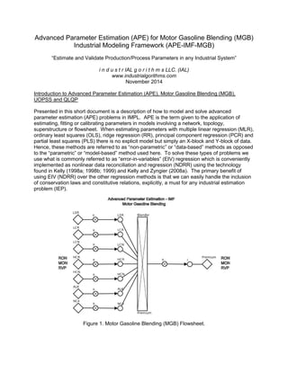
1. Advanced Parameter Estimation (APE) for Motor Gasoline Blending (MGB)
Industrial Modeling Framework (APE-IMF-MGB)
“Estimate and Validate Production/Process Parameters in any Industrial System”
i n d u s t r IAL g o r i t h m s LLC. (IAL)
www.industrialgorithms.com
November 2014
Introduction to Advanced Parameter Estimation (APE), Motor Gasoline Blending (MGB),
UOPSS and QLQP
Presented in this short document is a description of how to model and solve advanced
parameter estimation (APE) problems in IMPL. APE is the term given to the application of
estimating, fitting or calibrating parameters in models involving a network, topology,
superstructure or flowsheet. When estimating parameters with multiple linear regression (MLR),
ordinary least squares (OLS), ridge regression (RR), principal component regression (PCR) and
partial least squares (PLS) there is no explicit model but simply an X-block and Y-block of data.
Hence, these methods are referred to as “non-parametric” or “data-based” methods as opposed
to the “parametric” or “model-based” method used here. To solve these types of problems we
use what is commonly referred to as “error-in-variables” (EIV) regression which is conveniently
implemented as nonlinear data reconciliation and regression (NDRR) using the technology
found in Kelly (1998a; 1998b; 1999) and Kelly and Zyngier (2008a). The primary benefit of
using EIV (NDRR) over the other regression methods is that we can easily handle the inclusion
of conservation laws and constitutive relations, explicitly, a must for any industrial estimation
problem (IEP).
Figure 1. Motor Gasoline Blending (MGB) Flowsheet.

2. In order to demonstrate this, Figure 1 depicts a small but representative motor gasoline blending
(MGB) problem represented in our UOPSS flowsheet paradigm (Kelly, 2004; Kelly 2005;
Zyngier and Kelly, 2012). These types of blending problems are ubiquitous in oil-refining (Kelly
and Mann, 2003; Kelly 2006, Castillo et. al. 2013; Kelly et. al. 2014) where models relating
component recipes or flows (LSR, …, NC4) to component and product (Premium) properties
(RON, MON, RVP, etc.) are required for planning, scheduling, optimizing and controlling these
industrial systems. The UOPSS shapes shown in this figure are diamonds for perimeter unit-operations,
circles with and without “x”’s for outlet and inlet port-states respectively, a rectangle
with an “x” for a continuous-process unit-operation and the lines with arrow-heads for port-to-port
transfers or external streams and lines without arrow-heads for internal streams between
the unit-operation and the port-state.
The overall goal or purpose of this example is to use actual “end-of-blend report” (EBR) data for
thirty-three (33) blends or batches of premium motor gasoline and to estimate, fit or adapt linear
blending-values for each component and for each property i.e., 7 (components) * 3 (properties)
= 21 parameters or coefficients. These blending-values can then be used as the internal model
found in blend property controllers with on-line property measurements, instruments or
analyzers along with bias-updating (parameter-feedback) to effectively control these processes.
The EBR data is very common in blend-shops and reports the amount (volume or weight) of
each component used and the total amount of the product blended and has several measured
properties where RON, MON and RVP are the most common specifications but other properties
such as sulfur, olefins, aromatics content, distillation temperatures, etc. are also specified and
measured (Kelly et. al., 2014). There are essentially three (3) well-known nonlinear blending
models available such as the Ethyl, Dupont (Interaction) and Mobil Transformation methods but
these also require frequent calibration where their intrinsic predictive value over simply adapting
the linear blending-values from actual data is not understood to say the least.
Our novel approach here is to model each of the blends or batches as “scenarios” which are
conceptually identical to scenarios found in Scenario Optimization for example used to
effectively manage uncertainty i.e., to find a robust, reliable and resilient solution to a family of
possible situations. Here a scenario can be thought of as a “sample”, “survey” or “snapshot” of
the process or production at any instant of time in the past where a scenario is usually defined
for future events in planning and scheduling problems. As mentioned, since we have 33
samples or scenarios then technically there are 7 * 3 * 33 = 693 possible blending-values but
instead we common, link or match all of scenario blending-values together for a particular
stream so that we have only 7 * 3 = 21 blending-values (degrees-of-freedom, DoF) to estimate
where the other 672 blending-values are completely dependent (i.e., simple examples of linear
constitutive equations). How we do this in IMPL can be found in Appendix B under the
“Common Data” section. As any new blend is completed and/or when a past blend is deemed
to be too old or out-of-date, the set of scenarios can be modified or updated and the APE
process can be repeated in a rolling, receding or moving horizon estimation procedure (Kelly
and Zyngier, 2008b).
Industrial Modeling Framework (IMF), IMPL and SSIIMPLE
To implement the mathematical formulation of this and other systems, IAL offers a unique
approach and is incorporated into our Industrial Modeling Programming Language we call IMPL.
IMPL has its own modeling language called IML (short for Industrial Modeling Language) which
is a flat or text-file interface as well as a set of API's which can be called from any computer
programming language such as C, C++, Fortran, C#, VBA, Java (SWIG), Python (CTYPES)
and/or Julia (CCALL) called IPL (short for Industrial Programming Language) to both build the

3. model and to view the solution. Models can be a mix of linear, mixed-integer and nonlinear
variables and constraints and are solved using a combination of LP, QP, MILP and NLP solvers
such as COINMP, GLPK, LPSOLVE, SCIP, CPLEX, GUROBI, LINDO, XPRESS, CONOPT,
IPOPT, KNITRO and WORHP as well as our own implementation of SLP called SLPQPE
(Successive Linear & Quadratic Programming Engine) which is a very competitive alternative to
the other nonlinear solvers and embeds all available LP and QP solvers.
In addition and specific to DRR problems, we also have a special solver called SECQPE
standing for Sequential Equality-Constrained QP Engine which computes the least-squares
solution and a post-solver called SORVE standing for Supplemental Observability, Redundancy
and Variability Estimator to estimate the usual DRR statistics. SECQPE also includes a
Levenberg-Marquardt regularization method for nonlinear data regression problems and can be
presolved using SLPQPE i.e., SLPQPE warm-starts SECQPE. SORVE is run after the
SECQPE solver and also computes the well-known "maximum-power" gross-error statistics
(measurement and nodal/constraint tests) to help locate outliers, defects and/or faults i.e., mal-functions
in the measurement system and mis-specifications in the logging system.
The underlying system architecture of IMPL is called SSIIMPLE (we hope literally) which is short
for Server, Solvers, Interfacer (IML), Interacter (IPL), Modeler, Presolver Libraries and
Executable. The Server, Solvers, Presolver and Executable are primarily model or problem-independent
whereas the Interfacer, Interacter and Modeler are typically domain-specific i.e.,
model or problem-dependent. Fortunately, for most industrial planning, scheduling,
optimization, control and monitoring problems found in the process industries, IMPL's standard
Interfacer, Interacter and Modeler are well-suited and comprehensive to model the most difficult
of production and process complexities allowing for the formulations of straightforward
coefficient equations, ubiquitous conservation laws, rigorous constitutive relations, empirical
correlative expressions and other necessary side constraints.
User, custom, adhoc or external constraints can be augmented or appended to IMPL when
necessary in several ways. For MILP or logistics problems we offer user-defined constraints
configurable from the IML file or the IPL code where the variables and constraints are
referenced using unit-operation-port-state names and the quantity-logic variable types. It is also
possible to import a foreign *.ILP file (row-based MPS file) which can be generated by any
algebraic modeling language or matrix generator. This file is read just prior to generating the
matrix and before exporting to the LP, QP or MILP solver. For NLP or quality problems we offer
user-defined formula configuration in the IML file and single-value and multi-value function
blocks writable in C, C++ or Fortran. The nonlinear formulas may include intrinsic functions
such as EXP, LN, LOG, SIN, COS, TAN, MIN, MAX, IF, NOT, EQ, NE, LE, LT, GE, GT, AND,
OR, XOR and CIP, LIP, SIP and KIP (constant, linear and monotonic spline interpolations) as
well as user-written extrinsic functions (XFCN). It is also possible to import another type of
foreign file called the *.INL file where both linear and nonlinear constraints can be added easily
using new or existing IMPL variables.
Industrial modeling frameworks or IMF's are intended to provide a jump-start to an industrial
project implementation i.e., a pre-project if you will, whereby pre-configured IML files and/or IPL
code are available specific to your problem at hand. The IML files and/or IPL code can be
easily enhanced, extended, customized, modified, etc. to meet the diverse needs of your project
and as it evolves over time and use. IMF's also provide graphical user interface prototypes for
drawing the flowsheet as in Figure 1 and typical Gantt charts and trend plots to view the solution
of quantity, logic and quality time-profiles. Current developments use Python 2.3 and 2.7
integrated with open-source Gnome Dia and Matplotlib modules respectively but other

4. prototypes embedded within Microsoft Excel/VBA for example can be created in a
straightforward manner.
However, the primary purpose of the IMF's is to provide a timely, cost-effective, manageable
and maintainable deployment of IMPL to formulate and optimize complex industrial
manufacturing systems in either off-line or on-line environments. Using IMPL alone would be
somewhat similar (but not as bad) to learning the syntax and semantics of an AML as well as
having to code all of the necessary mathematical representations of the problem including the
details of digitizing your data into time-points and periods, demarcating past, present and future
time-horizons, defining sets, index-sets, compound-sets to traverse the network or topology,
calculating independent and dependent parameters to be used as coefficients and bounds and
finally creating all of the necessary variables and constraints to model the complex details of
logistics and quality industrial optimization problems. Instead, IMF's and IMPL provide, in our
opinion, a more elegant and structured approach to industrial modeling and solving so that you
can capture the benefits of advanced decision-making faster, better and cheaper.
Advanced Parameter Estimation (APE) and Motor Gasoline Blending (MGB) Synopsis
At this point we explore further the application of modeling and solving APE problems in IMPL.
The UOPSS shapes or objects arranged in the blend-shop flowsheet of Figure 1 can be found in
Appendix A we call the UPS file. A master IML file is found in Appendix B which configures
several calculations including the hypothetical blending-values (LSR_RON, …, NC4_RVP) from
which we simulate the actual Premium product or grade property values for RON, MON and
RVP where for RVP we simulate the typical (Chevron) blending-index of RVP^1.25. Scenario
1’s IML file (“S1:”) can be found in Appendix C where we use actual component recipes
(LSR=0.0911, …, NC4=0.1202) from an actual blend-shop. The other thirty-two (32) scenario
IML files for “S2:”, …, “S33:” are identical to Appendix C except that the actual component
recipes are different where Appendix B’s Case Data comments shows all of the actual scenario
recipes in table or matrix form. Although Normally distributed random noise could be added to
the simulated product properties in each scenario (see NOISESTD, NOISESEED and NRN)),
no noise was superimposed in order to better compare the regressed blending-values with the
simulated values.
The procedure to estimate the blending-values using the EBR data is to regress each property
individually in order to determine the individual “sum of squares of residuals” (SSR) which also
determines the “standard error” (SE). To do this in IMPL, the RONSE (Appendix B) is set to 1.0
while the MONSE and RVPSE are set to some large number such as 1E+20 and the SECQPE
solver is run which performs NDRR respecting equality constraints only (ignores inequality
constraints). The three SSR’s are 0.5100, 0.4501 and 0.0594 respectively where when we
divide the SSR’s by the nominal DoF of 32 this computes the SE where the inverse or reciprocal
is used as the 2-norm performance weight for the estimation (see Appendix C’s “Cost Data”).
The diagnostics are computed using SORVE which determines the observability of the
blending-values or coefficients (unmeasured or regressed variables), redundancy of the
measurements (measured or reconciled variables) and variances for both. Given the variances
we can compute the Student-t and Chi-Squared distribution statistics required by the data
reconciliation diagnostics known as the maximum-power measurement statistic, parameter
confidence-intervals and the global or objective function statistic. If significant autocorrelation is
detected in the residuals (measured minus predicted) such as detected by the Durbin-Watson
test for example then either a dynamic model needs to be configured using lagged or time-

5. shifted variables (explicit Euler’s method) or only steady-state data should be considered (Kelly
and Hedengren, 2013). Fortunately for this EBR data set, there is no autocorrelation present.
Table 1 shows the simulated versus regressed blending-values with 95% confidence-intervals
(CI’s) in parentheses. All of the blending-value coefficients are within their 95% CI’s except for
HCR which is somewhat related to the fact that there are only sixteen (16) scenarios with non-zero
HCR recipe or flow out of thirty-three (33). Although not shown, the RVP blending-values
are all within their CI’s comfortably.
Table 1. Simulated v. Regressed Blending-Value Parameters (95% Confidence-Intervals).
RON (Simulated) RON (Regressed) MON (Simulated) MON (Regressed)
LSR 74.80 75.95 (73.93,77.97) 71.20 72.27 (70.37,74.17)
LCR 97.40 96.89 (96.16,97.62) 90.90 90.43 (89.75,91.11)
LCN 80.70 79.65 (77.26,82.04) 78.50 77.50 (75.25,79.74)
HCR 103.00 102.04 (101.61,102.47) 93.00 92.12 (91.71,92.52)
HCN 89.60 91.90 (89.07,94.72) 80.50 82.66 (80.00,85.31)
ALK 95.30 95.03 (94.51,95.54) 92.20 91.93 (91.45,92.42)
NC4 96.00 95.01 (93.39,96.64) 90.50 89.56 (88.03,91.09)
An important feature of APE and NDRR is its ability to handle what is commonly referred to as
“missing-data”. Missing-data is the issue where not all of the X-block and Y-block data are
available. With most regression methods (excluding PCR and PLS), missing-data is handled
either by completing removing the observation, sample or scenario or “imputing” a value such
as using its mean. When missing-data is present in APE, we simply make the measured data
into unmeasured data whereby the NDRR will actually estimate or fit a reconciled/regressed
value using the inherent redundancy in the data and in the model. If we assume that the LSR
recipe or flow is missing in scenario “S1:” (see Appendix C’s Command Data), then we simply
set its lower and upper bounds to be some appropriate range. This then becomes a nonlinear
problem due to the flow times property bilinear term and SECQPE estimates its value to be
0.6613 (0.6546, 0.6681) where its measured value is 0.6582 and is clearly within its CI’s. If we
assume that the RON property in “S1:” is missing (see Appendix C’s Command Data), then we
simply set the target bound to our Non-Naturally Occurring Number (NNON=-99,999) which will
ignore this as a measurement. This is still a linear problem where SECQPE finds the RON
unmeasured value to be 92.60 (92.53, 92.68) where its measured value is 92.49.
In summary, it should be clear that IMPL can be used to model and solve advanced parameter
estimation (APE) problems which can also be considered as “Process or Production Analytics”
given that we are using prior engineering knowledge, process/production data and popular
statistics to identify and estimate these models that can then be used in industrial optimization
problems (IOP’s). Not only can we estimate process/production models that include a
flowsheet, nonlinearities, dynamics and missing-data using well-established statistical methods
such as EIV and NDRR but we are also able to provide the necessary diagnostic capability to
validate these models.
References
Kelly, J.D., "On finding the matrix projection in the data reconciliation solution", Computers and
Chemical Engineering, 1553, (1998a).

6. Kelly, J.D., "A regularization approach to the reconciliation of constrained data sets", Computers
and Chemical Engineering, 1771, (1998b).
Kelly, J.D., "Reconciliation of process data using other projection matrices", Computers and
Chemical Engineering, 785, (1999).
Kelly, J.D., Mann, J.M., "Crude-oil blend scheduling optimization: an application with multi-million
dollar benefits", Hydrocarbon Processing, June, 47, July, 72, (2003).
Kelly, J.D., "Production modeling for multimodal operations", Chemical Engineering Progress,
February, 44, (2004).
Kelly, J.D., "The unit-operation-stock superstructure (UOSS) and the quantity-logic-quality
paradigm (QLQP) for production scheduling in the process industries", In: MISTA 2005
Conference Proceedings, 327, (2005).
Kelly, J.D., "Logistics: the missing link in blend scheduling optimization", Hydrocarbon
Processing, June, 45, (2006).
Kelly, J.D., Zyngier, D., "A new and improved MILP formulation to optimize observability,
redundancy and precision for sensor network problems", American Institute of Chemical
Engineering Journal, 54, 1282, (2008a).
Kelly, J.D., Zyngier, D., "Continuously improve planning and scheduling models with parameter
feedback", FOCAPO 2008, July, (2008).
Zyngier, D., Kelly, J.D., "UOPSS: a new paradigm for modeling production planning and
scheduling systems", ESCAPE 22, June, (2012).
Castillo, P.A., Kelly, J.D., Mahalec, V., "Inventory pinch analysis for gasoline blend planning",
AIChE J., June, (2013).
Kelly, J.D., Hedengren, J.D., "A steady-state detection (SDD) algorithm to detect non-stationary
drifts in processes", Journal of Process Control, 23, 326, (2013).
Kelly, J.D., Menezes, B.C., Grossmann, I.E., “Distillation blending and cutpoint temperature
optimization using monotonic interpolation”, Industrial and Engineering Chemistry Research, 53,
15146-15156, (2014).
Appendix A – APE-IMF.UPS File
i M P l (c)
Copyright and Property of i n d u s t r I A L g o r i t h m s LLC.
checksum,73
!!!!!!!!!!!!!!!!!!!!!!!!!!!!!!!!!!!!!!!!!!!!!!!!!!!!!!!!!!!!!!
! Unit-Operation-Port-State-Superstructure (UOPSS) *.UPS File.
! (This file is automatically generated from the Python program IALConstructer.py)
!!!!!!!!!!!!!!!!!!!!!!!!!!!!!!!!!!!!!!!!!!!!!!!!!!!!!!!!!!!!!!
&sUnit,&sOperation,@sType,@sSubtype,@sUse
ALK,,perimeter,,
Blender,Premium,processc,blender%,
HCN,,perimeter,,
HCR,,perimeter,,
LCN,,perimeter,,
LCR,,perimeter,,
LSR,,perimeter,,
NC4,,perimeter,,

7. Premium,,perimeter,,
&sUnit,&sOperation,@sType,@sSubtype,@sUse
! Number of UO shapes = 9
&sAlias,&sUnit,&sOperation
ALLPARTS,ALK,
ALLPARTS,Blender,Premium
ALLPARTS,HCN,
ALLPARTS,HCR,
ALLPARTS,LCN,
ALLPARTS,LCR,
ALLPARTS,LSR,
ALLPARTS,NC4,
ALLPARTS,Premium,
&sAlias,&sUnit,&sOperation
&sUnit,&sOperation,&sPort,&sState,@sType,@sSubtype
ALK,,o,,out,
Blender,Premium,ALK,,in,
Blender,Premium,HCN,,in,
Blender,Premium,HCR,,in,
Blender,Premium,LCN,,in,
Blender,Premium,LCR,,in,
Blender,Premium,LSR,,in,
Blender,Premium,NC4,,in,
Blender,Premium,o,,out,
HCN,,o,,out,
HCR,,o,,out,
LCN,,o,,out,
LCR,,o,,out,
LSR,,o,,out,
NC4,,o,,out,
Premium,,i,,in,
&sUnit,&sOperation,&sPort,&sState,@sType,@sSubtype
! Number of UOPS shapes = 16
&sAlias,&sUnit,&sOperation,&sPort,&sState
ALLINPORTS,Blender,Premium,ALK,
ALLINPORTS,Blender,Premium,HCN,
ALLINPORTS,Blender,Premium,HCR,
ALLINPORTS,Blender,Premium,LCN,
ALLINPORTS,Blender,Premium,LCR,
ALLINPORTS,Blender,Premium,LSR,
ALLINPORTS,Blender,Premium,NC4,
ALLINPORTS,Premium,,i,
ALLOUTPORTS,ALK,,o,
ALLOUTPORTS,Blender,Premium,o,
ALLOUTPORTS,HCN,,o,
ALLOUTPORTS,HCR,,o,
ALLOUTPORTS,LCN,,o,
ALLOUTPORTS,LCR,,o,
ALLOUTPORTS,LSR,,o,
ALLOUTPORTS,NC4,,o,
&sAlias,&sUnit,&sOperation,&sPort,&sState
&sUnit,&sOperation,&sPort,&sState,&sUnit,&sOperation,&sPort,&sState
ALK,,o,,Blender,Premium,ALK,
Blender,Premium,o,,Premium,,i,
HCN,,o,,Blender,Premium,HCN,
HCR,,o,,Blender,Premium,HCR,
LCN,,o,,Blender,Premium,LCN,
LCR,,o,,Blender,Premium,LCR,
LSR,,o,,Blender,Premium,LSR,
NC4,,o,,Blender,Premium,NC4,
&sUnit,&sOperation,&sPort,&sState,&sUnit,&sOperation,&sPort,&sState
! Number of UOPSPSUO shapes = 8
&sAlias,&sUnit,&sOperation,&sPort,&sState,&sUnit,&sOperation,&sPort,&sState
ALLPATHS,ALK,,o,,Blender,Premium,ALK,
ALLPATHS,HCN,,o,,Blender,Premium,HCN,
ALLPATHS,HCR,,o,,Blender,Premium,HCR,
ALLPATHS,LCN,,o,,Blender,Premium,LCN,
ALLPATHS,LCR,,o,,Blender,Premium,LCR,
ALLPATHS,LSR,,o,,Blender,Premium,LSR,
ALLPATHS,NC4,,o,,Blender,Premium,NC4,
ALLPATHS,Blender,Premium,o,,Premium,,i,
&sAlias,&sUnit,&sOperation,&sPort,&sState,&sUnit,&sOperation,&sPort,&sState
Appendix B – APE-IMF.IML File
i M P l (c)
Copyright and Property of i n d u s t r I A L g o r i t h m s LLC.
!!!!!!!!!!!!!!!!!!!!!!!!!!!!!!!!!!!!!!!!!!!!!!!!!!!!!!!!!!!!!!!!!!!!!!!!!!!!!!!!
! Calculation Data (Parameters)
!!!!!!!!!!!!!!!!!!!!!!!!!!!!!!!!!!!!!!!!!!!!!!!!!!!!!!!!!!!!!!!!!!!!!!!!!!!!!!!!
&sCalc,@sValue
PERIOD,1.0
START,-PERIOD

8. BEGIN,0.0
END,1.0
DELTA,0.0
NOISESTD,0.0
NOISESEED,4*50+1
RONSE,0.5100 / 32
MONSE,0.4501 / 32
RVPSE,0.0594 / 32
! RON MON RVP
!LSR 74.80 71.20 14.80
!LCR 97.40 90.90 14.30
!LCN 80.70 78.50 12.20
!HCR 103.00 93.00 1.20
!HCN 89.60 80.50 1.70
!ALK 95.30 92.20 7.80
!NC4 96.00 90.50 52.00
LSR_RON,74.8
LCR_RON,97.40
LCN_RON,80.70
HCR_RON,103.00
HCN_RON,89.60
ALK_RON,95.30
NC4_RON,96.00
LSR_MON,71.20
LCR_MON,90.90
LCN_MON,78.50
HCR_MON,93.00
HCN_MON,80.50
ALK_MON,92.20
NC4_MON,90.50
! Transformed RVP (blending index).
LSR_RVP,(14.8)^1.25
LCR_RVP,(14.30)^1.25
LCN_RVP,(12.20)^1.25
HCR_RVP,(1.20)^1.25
HCN_RVP,(1.70)^1.25
ALK_RVP,(7.80)^1.25
NC4_RVP,(52.00)^1.25
&sCalc,@sValue
!!!!!!!!!!!!!!!!!!!!!!!!!!!!!!!!!!!!!!!!!!!!!!!!!!!!!!!!!!!!!!!!!!!!!!!!!!!!!!!!
! Chronological Data (Periods)
!!!!!!!!!!!!!!!!!!!!!!!!!!!!!!!!!!!!!!!!!!!!!!!!!!!!!!!!!!!!!!!!!!!!!!!!!!!!!!!!
@rPastTHD,@rFutureTHD,@rTPD
START,END,PERIOD
@rPastTHD,@rFutureTHD,@rTPD
!!!!!!!!!!!!!!!!!!!!!!!!!!!!!!!!!!!!!!!!!!!!!!!!!!!!!!!!!!!!!!!!!!!!!!!!!!!!!!!!
! Case Data (Prefixes)
!!!!!!!!!!!!!!!!!!!!!!!!!!!!!!!!!!!!!!!!!!!!!!!!!!!!!!!!!!!!!!!!!!!!!!!!!!!!!!!!
! LSR LCR LCN HCR HCN ALK NC4
! 1 0.0911 0.6582 0.1242 0.0000 0.0000 0.0000 0.1202
! 2 0.0838 0.6643 0.1231 0.0000 0.0000 0.0000 0.1224
! 3 0.1765 0.6524 0.0577 0.0000 0.0000 0.0000 0.1107
! 4 0.0562 0.6761 0.1496 0.0000 0.0000 0.0000 0.1140
! 5 0.1471 0.6721 0.0742 0.0000 0.0000 0.0000 0.1033
! 6 0.1287 0.6589 0.1040 0.0000 0.0000 0.0000 0.1049
! 7 0.0840 0.6604 0.1422 0.0000 0.0000 0.0000 0.1070
! 8 0.1494 0.6316 0.1044 0.0000 0.0000 0.0000 0.1112
! 9 0.1228 0.5424 0.1183 0.0000 0.0000 0.1072 0.1030
! 10 0.1074 0.6496 0.1083 0.0000 0.0000 0.0000 0.1284
! 11 0.1353 0.6340 0.0877 0.0000 0.0000 0.0000 0.1398
! 12 0.1266 0.6102 0.1510 0.0000 0.0000 0.0000 0.1089
! 13 0.0926 0.6420 0.1174 0.0000 0.0000 0.0000 0.1417
! 14 0.0889 0.6379 0.1306 0.0000 0.0000 0.0000 0.1396
! 15 0.0888 0.5772 0.0902 0.0000 0.0000 0.0841 0.1533
! 16 0.1430 0.4775 0.0268 0.0000 0.0000 0.2109 0.1388
! 17 0.0637 0.6158 0.1622 0.0000 0.0000 0.0364 0.1155
! 18 0.1260 0.1788 0.0000 0.4145 0.0810 0.0722 0.1242
! 19 0.0856 0.1304 0.0000 0.4503 0.0846 0.0949 0.1509
! 20 0.1443 0.2216 0.0000 0.3949 0.0239 0.1220 0.0900
! 21 0.0860 0.1935 0.0000 0.4013 0.0000 0.2614 0.0515
! 22 0.1298 0.2543 0.0000 0.4157 0.0397 0.0744 0.0828
! 23 0.1238 0.1237 0.0000 0.3926 0.0000 0.2963 0.0577
! 24 0.1080 0.2617 0.0000 0.4267 0.0352 0.1294 0.0345
! 25 0.0905 0.1434 0.0000 0.3886 0.0000 0.3080 0.0629
! 26 0.1039 0.2561 0.0000 0.4184 0.0343 0.1286 0.0543
! 27 0.0759 0.2758 0.0526 0.4302 0.0395 0.0821 0.0394
! 28 0.0762 0.2508 0.0256 0.4268 0.0000 0.1714 0.0450
! 29 0.0861 0.2494 0.0317 0.4373 0.0000 0.1555 0.0339
! 30 0.0896 0.2842 0.0262 0.4234 0.0742 0.0554 0.0427
! 31 0.0761 0.1692 0.0248 0.2484 0.0000 0.4332 0.0422
! 32 0.0601 0.1596 0.0248 0.2550 0.0000 0.4577 0.0421
! 33 0.0998 0.2885 0.0257 0.4168 0.0751 0.0559 0.0339
Include-@sFile_Name

9. APE-IMF-S1.iml
Include-@sFile_Name
Include-@sFile_Name
APE-IMF-S2.iml
Include-@sFile_Name
Include-@sFile_Name
APE-IMF-S3.iml
Include-@sFile_Name
Include-@sFile_Name
APE-IMF-S4.iml
Include-@sFile_Name
Include-@sFile_Name
APE-IMF-S5.iml
Include-@sFile_Name
Include-@sFile_Name
APE-IMF-S6.iml
Include-@sFile_Name
Include-@sFile_Name
APE-IMF-S7.iml
Include-@sFile_Name
Include-@sFile_Name
APE-IMF-S8.iml
Include-@sFile_Name
Include-@sFile_Name
APE-IMF-S9.iml
Include-@sFile_Name
Include-@sFile_Name
APE-IMF-S10.iml
Include-@sFile_Name
Include-@sFile_Name
APE-IMF-S11.iml
Include-@sFile_Name
Include-@sFile_Name
APE-IMF-S12.iml
Include-@sFile_Name
Include-@sFile_Name
APE-IMF-S13.iml
Include-@sFile_Name
Include-@sFile_Name
APE-IMF-S14.iml
Include-@sFile_Name
Include-@sFile_Name
APE-IMF-S15.iml
Include-@sFile_Name
Include-@sFile_Name
APE-IMF-S16.iml
Include-@sFile_Name
Include-@sFile_Name
APE-IMF-S17.iml
Include-@sFile_Name
Include-@sFile_Name
APE-IMF-S18.iml
Include-@sFile_Name
Include-@sFile_Name
APE-IMF-S19.iml
Include-@sFile_Name
Include-@sFile_Name
APE-IMF-S20.iml
Include-@sFile_Name
Include-@sFile_Name
APE-IMF-S21.iml
Include-@sFile_Name
Include-@sFile_Name
APE-IMF-S22.iml
Include-@sFile_Name
Include-@sFile_Name
APE-IMF-S23.iml
Include-@sFile_Name
Include-@sFile_Name
APE-IMF-S24.iml
Include-@sFile_Name

10. Include-@sFile_Name
APE-IMF-S25.iml
Include-@sFile_Name
Include-@sFile_Name
APE-IMF-S26.iml
Include-@sFile_Name
Include-@sFile_Name
APE-IMF-S27.iml
Include-@sFile_Name
Include-@sFile_Name
APE-IMF-S28.iml
Include-@sFile_Name
Include-@sFile_Name
APE-IMF-S29.iml
Include-@sFile_Name
Include-@sFile_Name
APE-IMF-S30.iml
Include-@sFile_Name
Include-@sFile_Name
APE-IMF-S31.iml
Include-@sFile_Name
Include-@sFile_Name
APE-IMF-S32.iml
Include-@sFile_Name
Include-@sFile_Name
APE-IMF-S33.iml
Include-@sFile_Name
!!!!!!!!!!!!!!!!!!!!!!!!!!!!!!!!!!!!!!!!!!!!!!!!!!!!!!!!!!!!!!!!!!!!!!!!!!!!!!!!
! Common Data (Parities)
!!!!!!!!!!!!!!!!!!!!!!!!!!!!!!!!!!!!!!!!!!!!!!!!!!!!!!!!!!!!!!!!!!!!!!!!!!!!!!!!
&sUnit,&sOperation,&sPort,&sState,&sQuality,@sType,&sUnit,&sOperation,&sPort,&sState,&sQuality,@sType
LSR,,o,,RON,PP,
LCR,,o,,RON,PP,
LCN,,o,,RON,PP,
HCR,,o,,RON,PP,
HCN,,o,,RON,PP,
ALK,,o,,RON,PP,
NC4,,o,,RON,PP,
LSR,,o,,MON,PP,
LCR,,o,,MON,PP,
LCN,,o,,MON,PP,
HCR,,o,,MON,PP,
HCN,,o,,MON,PP,
ALK,,o,,MON,PP,
NC4,,o,,MON,PP,
LSR,,o,,RVP,PP,
LCR,,o,,RVP,PP,
LCN,,o,,RVP,PP,
HCR,,o,,RVP,PP,
HCN,,o,,RVP,PP,
ALK,,o,,RVP,PP,
NC4,,o,,RVP,PP,
&sUnit,&sOperation,&sPort,&sState,&sQuality,@sType,&sUnit,&sOperation,&sPort,&sState,&sQuality,@sType
Appendix C – APE-IMF-S1.IML File
i M P l (c)
Copyright and Property of i n d u s t r I A L g o r i t h m s LLC.
!!!!!!!!!!!!!!!!!!!!!!!!!!!!!!!!!!!!!!!!!!!!!!!!!!!!!!!!!!!!!!!!!!!!!!!!!!!!!!!!
! Case Data (Prefixes)
!!!!!!!!!!!!!!!!!!!!!!!!!!!!!!!!!!!!!!!!!!!!!!!!!!!!!!!!!!!!!!!!!!!!!!!!!!!!!!!!
&sScenario
S1:
&sScenario
!!!!!!!!!!!!!!!!!!!!!!!!!!!!!!!!!!!!!!!!!!!!!!!!!!!!!!!!!!!!!!!!!!!!!!!!!!!!!!!!
! Calculation Data (Parameters)
!!!!!!!!!!!!!!!!!!!!!!!!!!!!!!!!!!!!!!!!!!!!!!!!!!!!!!!!!!!!!!!!!!!!!!!!!!!!!!!!
&sCalc,@sValue
PERIOD,1.0
START,-PERIOD
BEGIN,0.0
END,1.0
! Measured/fixed component recipes.
LSR,0.0911
LCR,0.6582

11. LCN,0.1242
HCR,0.0000
HCN,0.0000
ALK,0.0000
NC4,0.1202
! Simulated properties.
NOISE,2.0 * (NRN(NOISESEED) - 0.5) * NOISESTD
RON,LSR*LSR_RON+ LCR*LCR_RON+ LCN*LCN_RON+ HCR*HCR_RON+ HCN*HCN_RON+ ALK*ALK_RON+ NC4*NC4_RON+ NOISE
MON,LSR*LSR_MON+ LCR*LCR_MON+ LCN*LCN_MON+ HCR*HCR_MON+ HCN*HCN_MON+ ALK*ALK_MON+ NC4*NC4_MON+ NOISE
RVP,LSR*LSR_RVP+ LCR*LCR_RVP+ LCN*LCN_RVP+ HCR*HCR_RVP+ HCN*HCN_RVP+ ALK*ALK_RVP+ NC4*NC4_RVP+ NOISE
&sCalc,@sValue
!!!!!!!!!!!!!!!!!!!!!!!!!!!!!!!!!!!!!!!!!!!!!!!!!!!!!!!!!!!!!!!!!!!!!!!!!!!!!!!!
! Construction Data (Pointers)
!!!!!!!!!!!!!!!!!!!!!!!!!!!!!!!!!!!!!!!!!!!!!!!!!!!!!!!!!!!!!!!!!!!!!!!!!!!!!!!!
Include-@sFile_Name
APE-IMF.ups
Include-@sFile_Name
!!!!!!!!!!!!!!!!!!!!!!!!!!!!!!!!!!!!!!!!!!!!!!!!!!!!!!!!!!!!!!!!!!!!!!!!!!!!!!!!
! Capacity Data (Prototypes)
!!!!!!!!!!!!!!!!!!!!!!!!!!!!!!!!!!!!!!!!!!!!!!!!!!!!!!!!!!!!!!!!!!!!!!!!!!!!!!!!
&sUnit,&sOperation,@rRate_Lower,@rRate_Upper
ALLPARTS,0.0,1000.0
&sUnit,&sOperation,@rRate_Lower,@rRate_Upper
&sUnit,&sOperation,&sPort,&sState,@rTeeRate_Lower,@rTeeRate_Upper
ALLINPORTS,0.0,1000.0
ALLOUTPORTS,0.0,1000.0
&sUnit,&sOperation,&sPort,&sState,@rTeeRate_Lower,@rTeeRate_Upper
&sUnit,&sOperation,&sPort,&sState,@rTotalRate_Lower,@rTotalRate_Upper
ALLINPORTS,0.0,1000.0
ALLOUTPORTS,0.0,1000.0
&sUnit,&sOperation,&sPort,&sState,@rTotalRate_Lower,@rTotalRate_Upper
&sUnit,&sOperation,&sPort,&sState,@rYield_Lower,@rYield_Upper,@rYield_Fixed
ALLINPORTS,0.0,1.0
ALLOUTPORTS,0.0,1.0
&sUnit,&sOperation,&sPort,&sState,@rYield_Lower,@rYield_Upper,@rYield_Fixed
!!!!!!!!!!!!!!!!!!!!!!!!!!!!!!!!!!!!!!!!!!!!!!!!!!!!!!!!!!!!!!!!!!!!!!!!!!!!!!!!
! Constituent Data (Properties)
!!!!!!!!!!!!!!!!!!!!!!!!!!!!!!!!!!!!!!!!!!!!!!!!!!!!!!!!!!!!!!!!!!!!!!!!!!!!!!!!
&sProperty
RON
MON
RVP
&sProperty
&sUnit,&sOperation,&sPort,&sState,&sProperty,@rProperty_Lower,@rProperty_Upper,@rProperty_Target
ALLINPORTS,RON,0.0,200.0
ALLINPORTS,MON,0.0,200.0
ALLINPORTS,RVP,0.0,200.0
ALLOUTPORTS,RON,0.0,200.0
ALLOUTPORTS,MON,0.0,200.0
ALLOUTPORTS,RVP,0.0,200.0
&sUnit,&sOperation,&sPort,&sState,&sProperty,@rProperty_Lower,@rProperty_Upper,@rProperty_Target
!!!!!!!!!!!!!!!!!!!!!!!!!!!!!!!!!!!!!!!!!!!!!!!!!!!!!!!!!!!!!!!!!!!!!!!!!!!!!!!!
! Cost Data (Pricing)
!!!!!!!!!!!!!!!!!!!!!!!!!!!!!!!!!!!!!!!!!!!!!!!!!!!!!!!!!!!!!!!!!!!!!!!!!!!!!!!!
&sUnit,&sOperation,&sPort,&sState,&sProperty,@rPropertyPro_Weight,@rPropertyPer1_Weight,@rPropertyPer2_Weight,@rPropertyPen_Weigh
t
Premium,,i,,RON,,,1.0/RONSE
Premium,,i,,MON,,,1.0/MONSE
Premium,,i,,RVP,,,1.0/RVPSE
&sUnit,&sOperation,&sPort,&sState,&sProperty,@rPropertyPro_Weight,@rPropertyPer1_Weight,@rPropertyPer2_Weight,@rPropertyPen_Weigh
t
!!!!!!!!!!!!!!!!!!!!!!!!!!!!!!!!!!!!!!!!!!!!!!!!!!!!!!!!!!!!!!!!!!!!!!!!!!!!!!!!
! Command Data (Future Provisos)
!!!!!!!!!!!!!!!!!!!!!!!!!!!!!!!!!!!!!!!!!!!!!!!!!!!!!!!!!!!!!!!!!!!!!!!!!!!!!!!!
&sUnit,&sOperation,@rSetup_Lower,@rSetup_Upper,@rBegin_Time,@rEnd_Time
ALLPARTS,1,1,BEGIN,END
&sUnit,&sOperation,@rSetup_Lower,@rSetup_Upper,@rBegin_Time,@rEnd_Time
&sUnit,&sOperation,&sPort,&sState,&sUnit,&sOperation,&sPort,&sState,@rSetup_Lower,@rSetup_Upper,@rBegin_Time,@rEnd_Time
ALLPATHS,1,1,BEGIN,END
&sUnit,&sOperation,&sPort,&sState,&sUnit,&sOperation,&sPort,&sState,@rSetup_Lower,@rSetup_Upper,@rBegin_Time,@rEnd_Time
&sUnit,&sOperation,&sPort,&sState,@rTotalRate_Lower,@rTotalRate_Upper,@rTotalRate_Target,@rBegin_Time,@rEnd_Time
LSR,,o,,MAX(LSR-DELTA;0.0),LSR+DELTA,,BEGIN,END
! Set lower and upper bounds if LCR flow measurement is missing (not available).
!LCR,,o,,0.0,1.0,,BEGIN,END
LCR,,o,,MAX(LCR-DELTA;0.0),LCR+DELTA,,BEGIN,END

12. LCN,,o,,MAX(LCN-DELTA;0.0),LCN+DELTA,,BEGIN,END
HCR,,o,,MAX(HCR-DELTA;0.0),HCR+DELTA,,BEGIN,END
HCN,,o,,MAX(HCN-DELTA;0.0),HCN+DELTA,,BEGIN,END
ALK,,o,,MAX(ALK-DELTA;0.0),ALK+DELTA,,BEGIN,END
NC4,,o,,MAX(NC4-DELTA;0.0),NC4+DELTA,,BEGIN,END
&sUnit,&sOperation,&sPort,&sState,@rTotalRate_Lower,@rTotalRate_Upper,@rTotalRate_Target,@rBegin_Time,@rEnd_Time
&sUnit,&sOperation,&sPort,&sState,&sProperty,@rProperty_Lower,@rProperty_Upper,@rProperty_Target,@rBegin_Time,@rEnd_Time
! Set target bound to RNNON if RON property measurement is missing (not available).
!Premium,,i,,RON,0.0,200.0,-99999,BEGIN,END
Premium,,i,,RON,0.0,200.0,RON,BEGIN,END
Premium,,i,,MON,0.0,200.0,MON,BEGIN,END
Premium,,i,,RVP,0.0,200.0,RVP,BEGIN,END
&sUnit,&sOperation,&sPort,&sState,&sProperty,@rProperty_Lower,@rProperty_Upper,@rProperty_Target,@rBegin_Time,@rEnd_Time