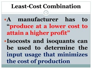
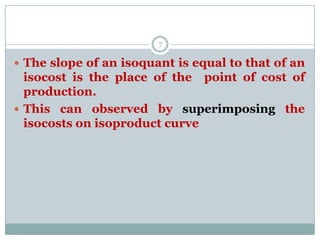
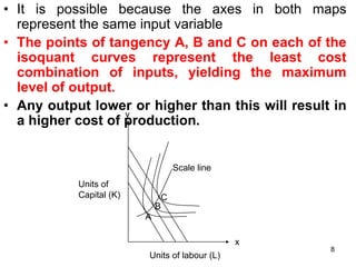
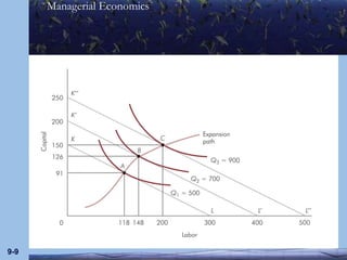
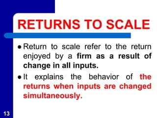
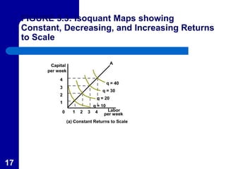
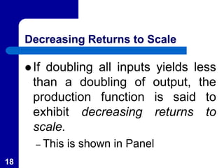
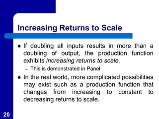
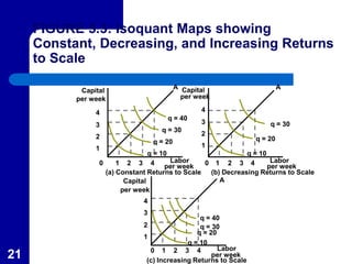
This document discusses different concepts in production economics including isocosts, least-cost input combinations, and returns to scale. It defines isocosts as cost curves that represent combinations of inputs that cost the same amount. Least-cost combinations are determined by superimposing isocost and isoquant curves to find points of tangency. Returns to scale refer to how output changes with proportional input changes. Constant returns mean output doubles with doubled inputs. Decreasing returns mean less than doubled output, while increasing returns mean more than doubled output.

1. Dr.K.Baranidharan
Present by…

2. Engineering
Economics &
Financial
Accountingment
Ee&fa
218 August 2013

3. INDEX
•Isocosts
•Least-cost Combination Of
Inputs
•Cobb-Douglas production
function
•Law of Return to Scale

4. ISOCOSTS
 Isocosts refer to the cost curve that
represents the combination of inputs
that will cost a producer the same
amount of money.
 Isocosts denotes IQ2a particular level of
total cost for a given level of
production.
 The level of production changes, the total
cost changes and, thus the isocosts
curve moves upwards
4

5. The total cost as represented by each cost
curve, is calculated by multiplying the
quantity of each input factor with its
respective price.
The three
download
sloping straight
line cost curves
(assuming that
the input prices
are fixed, no
quantity
discount are
available) each
costing Rs.1.0
lakh, Rs.1.5 lakh
and Rs.2.0 lakh
for the output
leavels of
20,000-30,000
and 40,000
units.
c
a
p
i
t
a
l
Labour
I
C
=
1
.
0
I
C
=
1
.
5
I
C
=
2
.
0
5

6. Least-Cost Combination
A manufacturer has to
“produce at a lower cost to
attain a higher profit”
Isocosts and isoquants can
be used to determine the
input usage that minimizes
the cost of production
6

7.  The slope of an isoquant is equal to that of an
isocost is the place of the point of cost of
production.
 This can observed by superimposing the
isocosts on isoproduct curve
7

8. • It is possible because the axes in both maps
represent the same input variable
• The points of tangency A, B and C on each of the
isoquant curves represent the least cost
combination of inputs, yielding the maximum
level of output.
• Any output lower or higher than this will result in
a higher cost of production.
Units of
Capital (K)
x
y
Units of labour (L)
A
B
C
Scale line
8

9. Managerial EconomicsManagerial Economics
9-9

10. Dr.K.Baranidharan
THANK YOU

11. Dr.K.Baranidharan
Present by…

12. Engineering
Economics &
Financial
Accountingment
Ee&fa
1218 August 2013

13. RETURNS TO SCALE
 Return to scale refer to the return
enjoyed by a firm as a result of
change in all inputs.
 It explains the behavior of the
returns when inputs are changed
simultaneously.
13

14. Returns to Scale
 Returns to scale is the rate at
which output increases in
response to proportional
increases in all inputs.
 In the eighteenth century Adam
Smith became aware of this concept
when he studied the production of
pins.14

15. Returns to Scale
 Adam Smith identified two forces that
come into play when all inputs are
increased.
– A doubling of inputs permits a greater
“division of labor” allowing persons to
specialize in the production of specific pin
parts.
– This specialization may increase efficiency
enough to more than double output.
15

16. Constant Returns to Scale
 A production function is said to
exhibit constant returns to scale
if a doubling of all inputs results
in a precise doubling of output.
– This situation is shown in Panel .
16

17. Capital
per week
4
A
3
2
1
Labor
per week1 2 3
(a) Constant Returns to Scale
40
FIGURE 5.3: Isoquant Maps showing
Constant, Decreasing, and Increasing Returns
to Scale
q = 10
q = 20
q = 30
q = 40
17

18. Decreasing Returns to Scale
 If doubling all inputs yields less
than a doubling of output, the
production function is said to
exhibit decreasing returns to
scale.
– This is shown in Panel
18

19. Capital
per week
4
A
3
2
1
Labor
per week1 2 3
(a) Constant Returns to Scale
40
Capital
per week
4
A
3
2
1
Labor
per week1 2 3
(b) Decreasing Returns to Scale
40
FIGURE 5.3: Isoquant Maps showing
Constant, Decreasing, and Increasing Returns
to Scale
q = 10 q = 10
q = 20q = 20
q = 30
q = 30
q = 40
19

20. Increasing Returns to Scale
 If doubling all inputs results in more than a
doubling of output, the production function
exhibits increasing returns to scale.
– This is demonstrated in Panel
 In the real world, more complicated possibilities
may exist such as a production function that
changes from increasing to constant to
decreasing returns to scale.
20

21. Capital
per week
4
A
q = 10
3
2
1
Labor
per week1 2 3
(a) Constant Returns to Scale
40
Capital
per week
4
A
3
2
1
Labor
per week
1 2 3
(c) Increasing Returns to Scale
40
Capital
per week
4
A
3
2
1
Labor
per week1 2 3
(b) Decreasing Returns to Scale
40
FIGURE 5.3: Isoquant Maps showing
Constant, Decreasing, and Increasing Returns
to Scale
q = 10 q = 10
q = 20
q = 20q = 20
q = 30
q = 30
q = 30
q = 40
q = 40
21

22. Dr.K.Baranidharan
THANK YOU