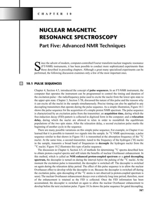
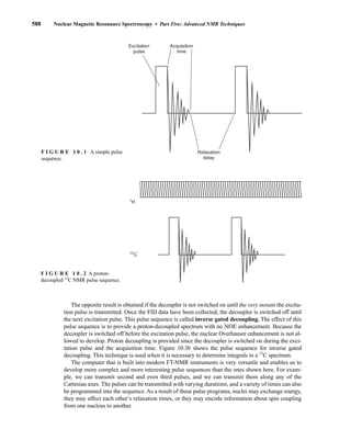
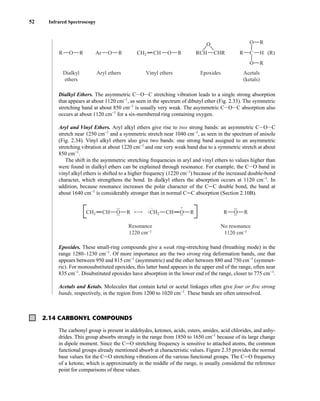
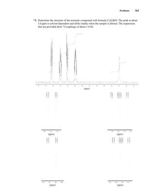
This document is an excerpt from the textbook Introduction to Spectroscopy by Donald L. Pavia, Gary M. Lampman, George S. Kriz, and James R. Vyvyan. It provides an overview of the contents of the textbook, which covers various spectroscopic techniques including infrared spectroscopy, nuclear magnetic resonance spectroscopy, and mass spectrometry. The textbook has been updated for the fourth edition with expanded discussions of NMR coupling constant analysis, solvent effects in NMR, determining stereochemistry with NMR, and mass spectrometry. It aims to teach students both how to interpret spectra and basic theoretical concepts in spectroscopy.


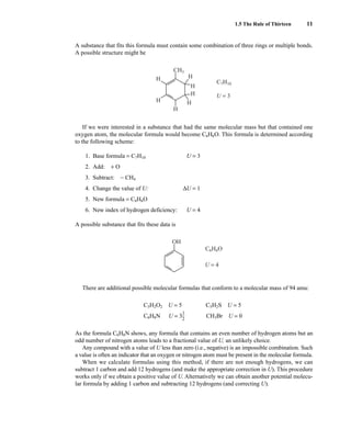

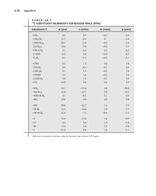
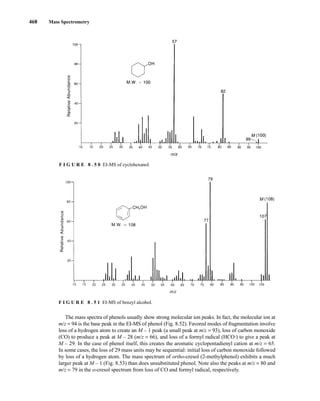
![105
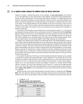
C H A P T E R 3
NUCLEAR MAGNETIC RESONANCE
SPECTROSCOPY
Part One: Basic Concepts
N
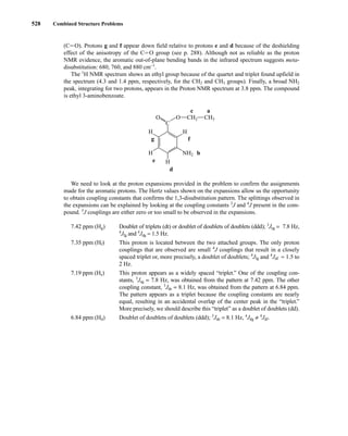
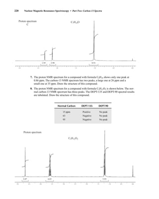
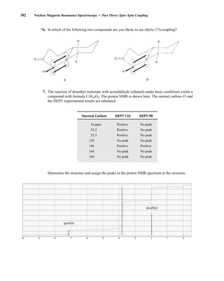
uclear magnetic resonance (NMR) is a spectroscopic method that is even more important
to the organic chemist than infrared spectroscopy. Many nuclei may be studied by NMR
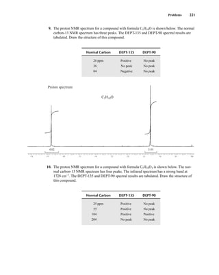
techniques, but hydrogen and carbon are most commonly available. Whereas infrared (IR)
spectroscopy reveals the types of functional groups present in a molecule, NMR gives information
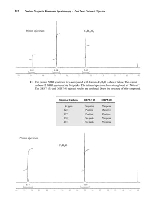
about the number of magnetically distinct atoms of the type being studied. When hydrogen nuclei
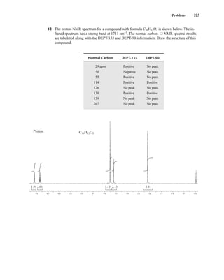
(protons) are studied, for instance, one can determine the number of each of the distinct types of
hydrogen nuclei as well as obtain information regarding the nature of the immediate environment of
each type. Similar information can be determined for the carbon nuclei. The combination of IR and
NMR data is often sufficient to determine completely the structure of an unknown molecule.
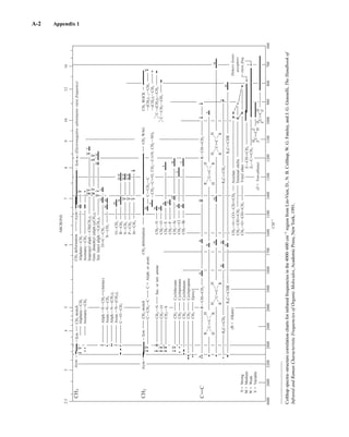
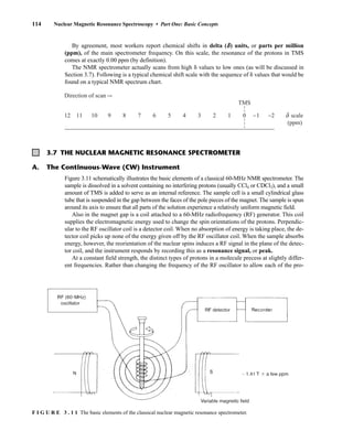
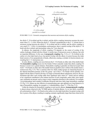
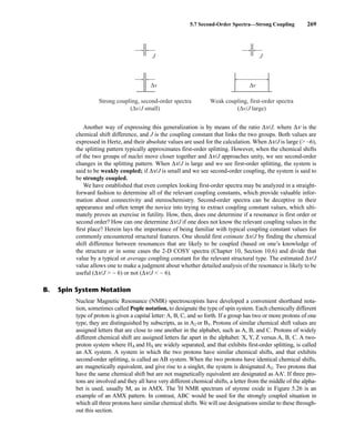
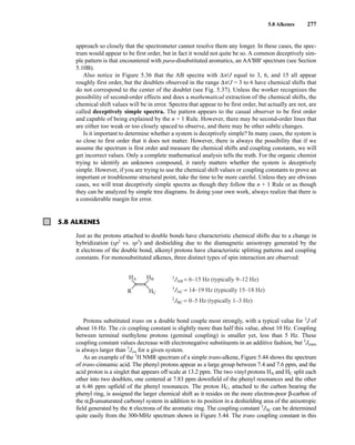
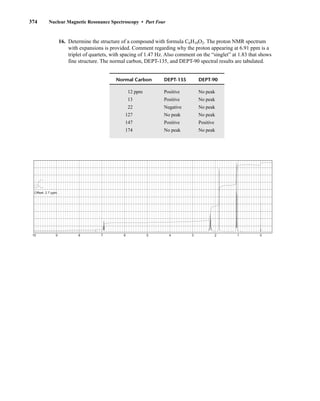
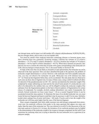
3.1 NUCLEAR SPIN STATES
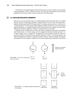
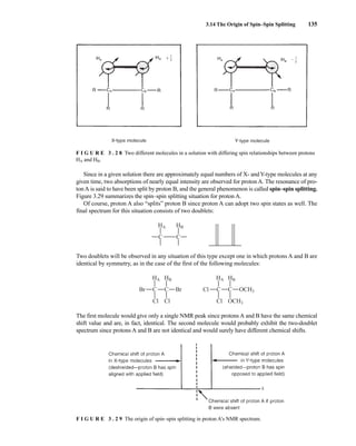
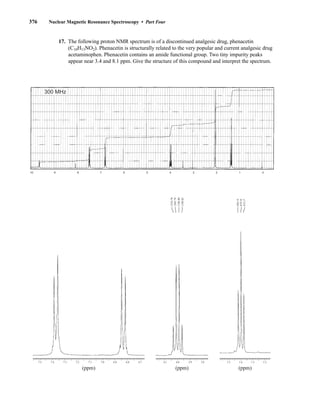
Many atomic nuclei have a property called spin: the nuclei behave as if they were spinning. In fact,
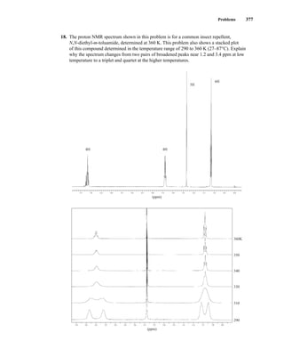
any atomic nucleus that possesses either odd mass, odd atomic number, or both has a quantized spin
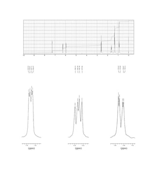
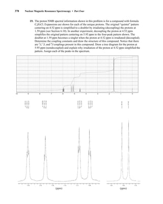
angular momentum and a magnetic moment. The more common nuclei that possess spin include
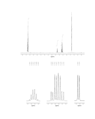
1
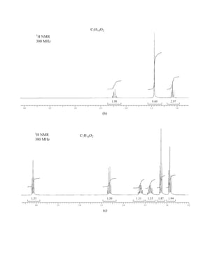
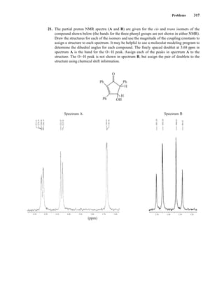
1H, 2
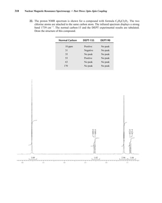
1H, 13
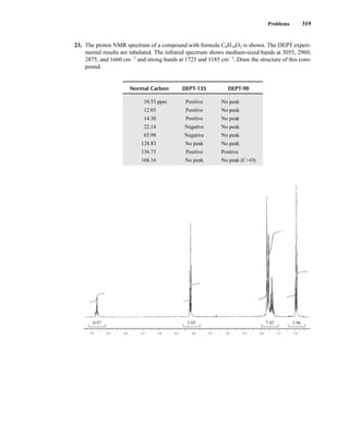
6C, 14
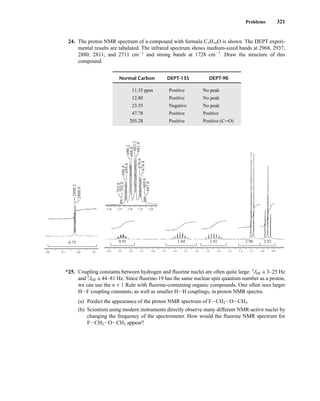
7N, 17
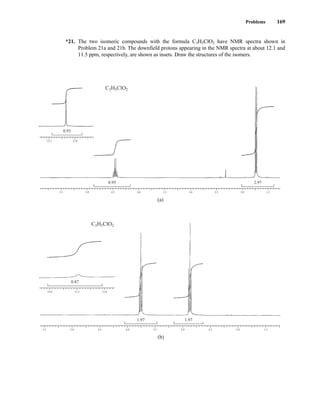
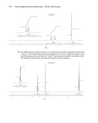
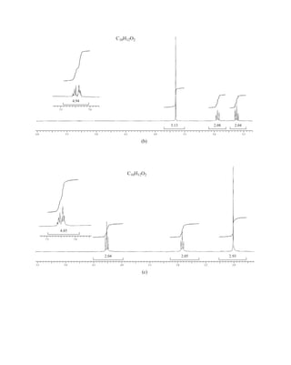
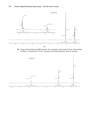
8O, and 19
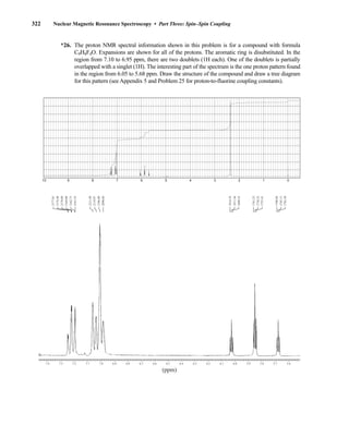
9F. Notice that the nuclei of the ordinary (most abundant) isotopes of car-
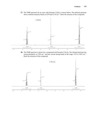
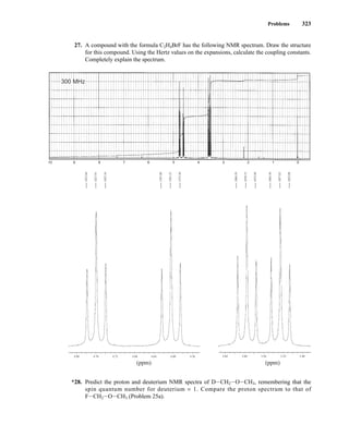
bon and oxygen, 12
6C and 16
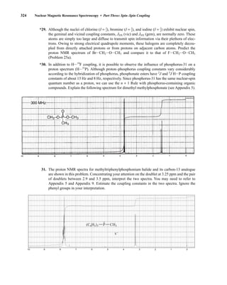
8O, are not included among those with the spin property. However, the nu-
cleus of the ordinary hydrogen atom, the proton, does have spin. For each nucleus with spin, the
number of allowed spin states it may adopt is quantized and is determined by its nuclear spin quan-
tum number I. For each nucleus, the number I is a physical constant, and there are 2I + 1 allowed spin
states with integral differences ranging from +I to −I. The individual spin states fit into the sequence
+I, (I − 1), . . . , (−I + 1), −I Equation 3.1
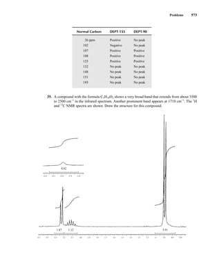
For instance, a proton (hydrogen nucleus) has the spin quantum number I = ⎯
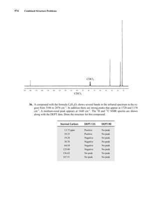
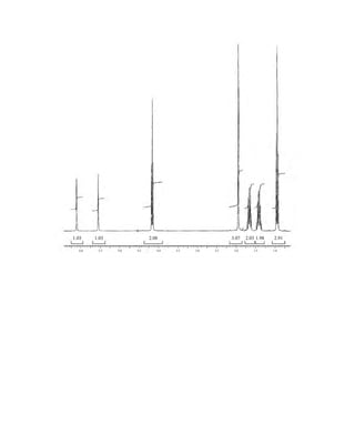
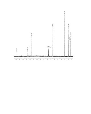
1
2
⎯ and has two allowed spin
states [2(⎯
1
2
⎯) + 1 = 2] for its nucleus: −⎯
1
2
⎯ and +⎯
1
2
⎯. For the chlorine nucleus, I = ⎯
3
2
⎯ and there are four allowed
spin states [2(⎯
3
2
⎯) + 1 = 4]: −⎯
3
2
⎯, −⎯
1
2
⎯, +⎯
1
2
⎯, and +⎯
3
2
⎯. Table 3.1 gives the spin quantum numbers of several nuclei.
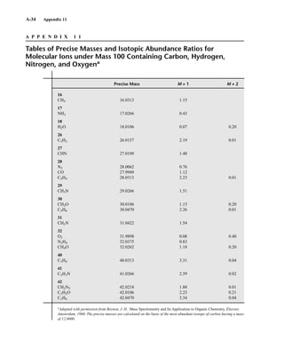
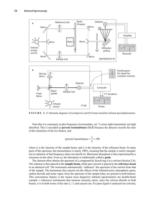
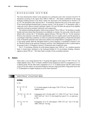
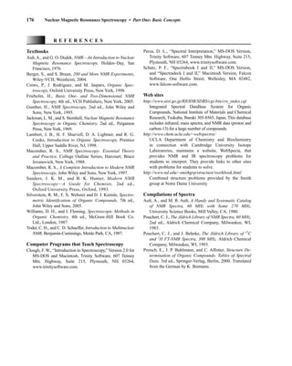
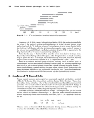
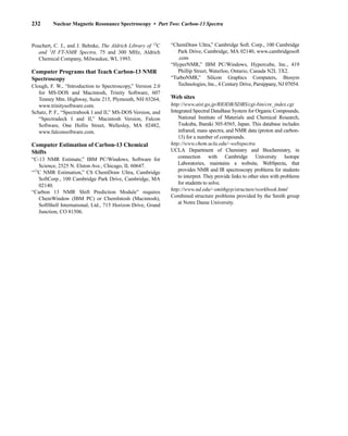
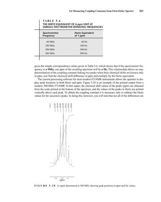
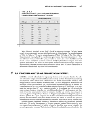
TA B L E 3 . 1
SPIN QUANTUM NUMBERS OF SOME COMMON NUCLEI
Element 1
1H 2
1H 12
6C 13
6C 14
7N 16
8O 17
8O 19
9F 31
15P 35
17Cl
Nuclear spin
quantum number ⎯
1
2
⎯ 1 0 ⎯
1
2
⎯ 1 0 ⎯
5
2
⎯ ⎯
1
2
⎯ ⎯
1
2
⎯ ⎯
2
3
⎯
Number of
spin states 2 3 0 2 3 0 6 2 2 4
14782_03_Ch3_p105-176.pp2.qxd 2/1/08 10:56 PM Page 105](https://image.slidesharecdn.com/introductiontospectroscopy4ebypavia-240123161815-89f06477/85/Introduction-to-Spectroscopy-4e-by-Pavia-pdf-122-320.jpg)
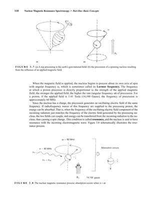
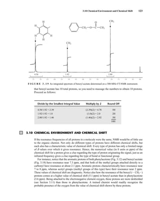
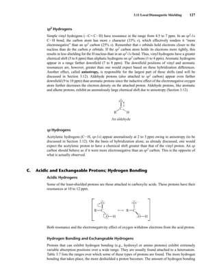
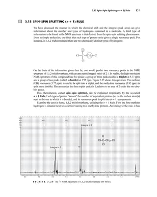

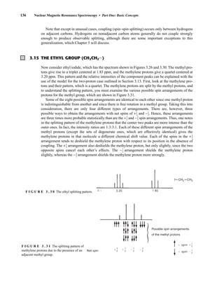
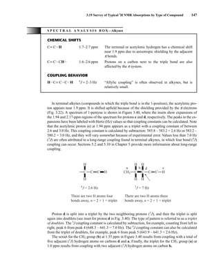
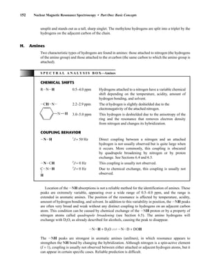
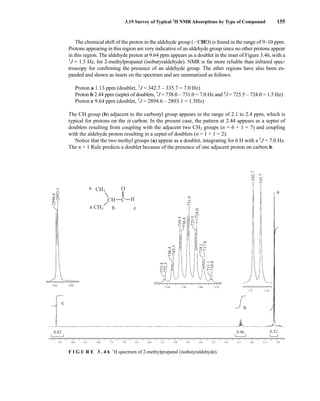

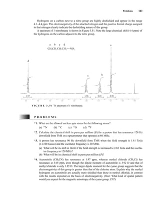
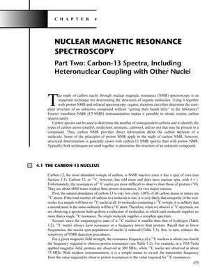
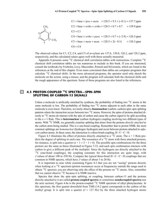
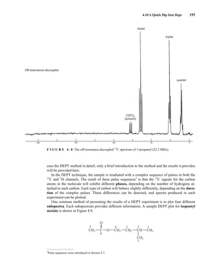
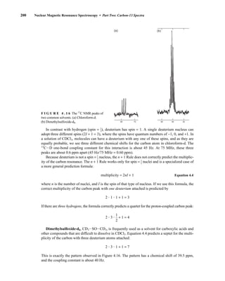
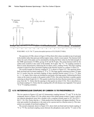
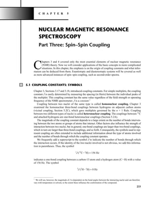
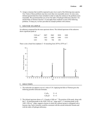
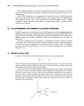
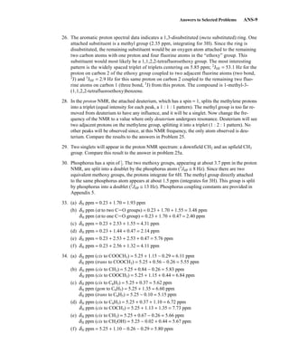
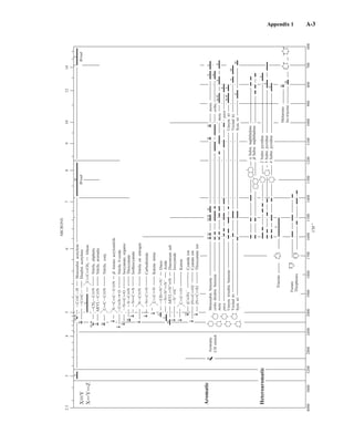
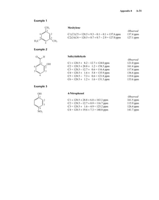
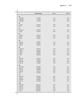
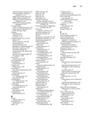
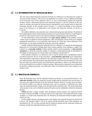
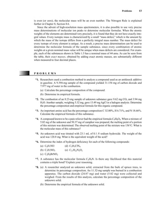
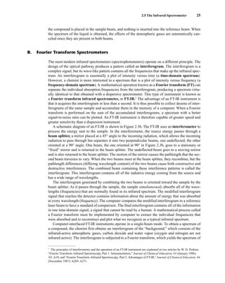
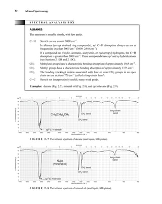
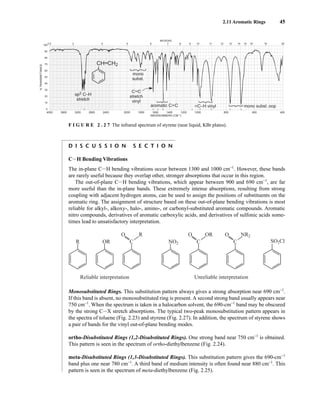
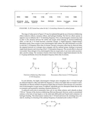
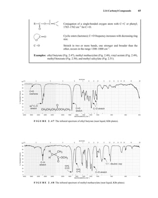
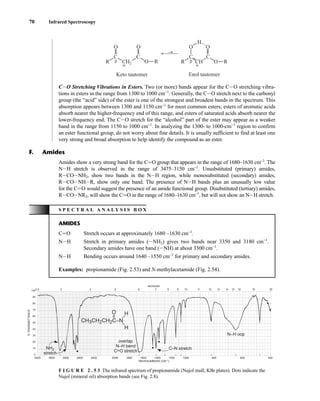
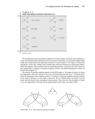
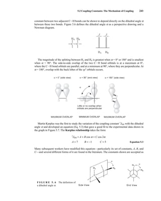
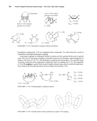
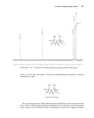
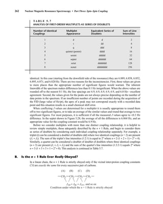
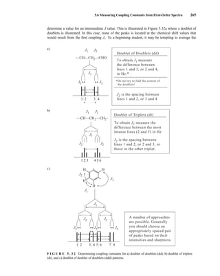
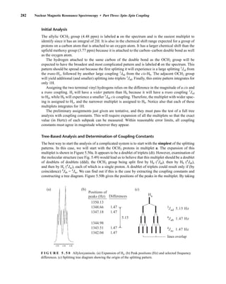
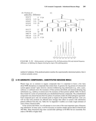
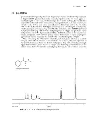
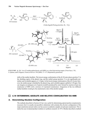
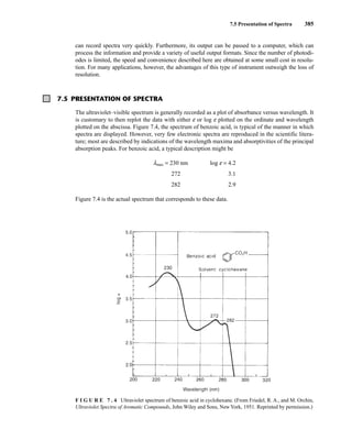
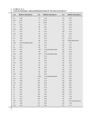
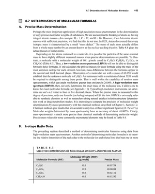
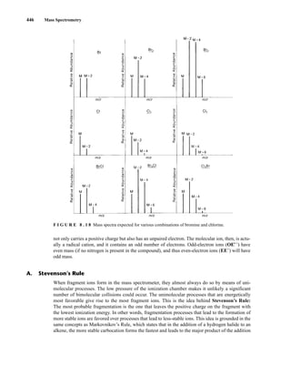
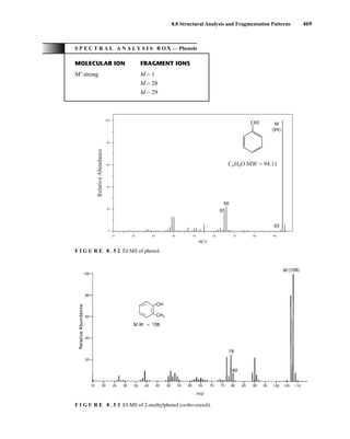
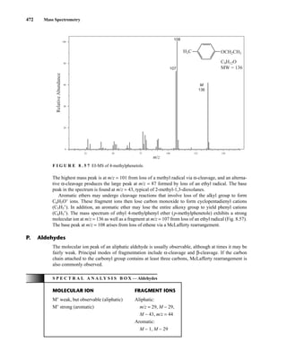
![At the bottom of Figure 5.2a is the favored ground state for the 13
CI1
H bond. In this arrange-
ment, the carbon nucleus is in its lowest energy state [spin (1
H) = +1/2], and all of the spins, both
nuclear and electronic, are paired, resulting in the lowest energy for the system. The spin of the nu-
cleus of the hydrogen atom is opposed to the spin of the 13
C nucleus. A higher energy results for the
system if the spin of the hydrogen is reversed [spin (1
H) = –1/2]. This less-favored ground state is
shown at the bottom of Figure 5.2b.
Now, assume that the carbon nucleus undergoes transition and inverts its spin. The excited state
that results from the less-favored ground state (seen at the top of Fig. 5.2b) turns out to have a lower
energy than the one resulting from the favored ground state (top of Fig. 5.2a) because all of its nu-
clear and electronic spins are paired. Thus, we see two different transitions for the 13
C nucleus
[spin(13
C) = +1/2], depending on the spin of the attached hydrogen. As a result, in a proton-coupled
NMR spectrum a doublet is observed for a methine carbon (13
CI1
H).
236 Nuclear Magnetic Resonance Spectroscopy • Part Three: Spin–Spin Coupling
Carbon nucleus
undergoes transition
Favored
ground state
H — 13
C
Carbon nucleus
undergoes transition
Less-favored
ground state
H — 13
C
= Carbon nucleus
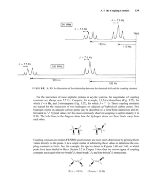
= Hydrogen nucleus
= Electrons
(a) (b)
F I G U R E 5 . 2 The two different energy transitions for a 13
C nucleus in a CIH bond. (a) The favored
ground state (all spins paired); (b) the less-favored ground state (impossible to pair all spins).
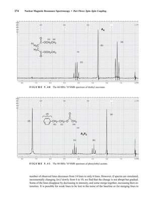
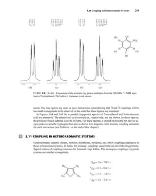
Two-bond couplings are quite common in NMR spectra. They are usually called geminal cou-
plings because the two nuclei that interact are attached to the same central atom (Latin gemini =
“twins”). Two-bond coupling constants are abbreviated 2
J. They occur in carbon compounds
whenever two or more spin-active atoms are attached to the same carbon atom. Table 5.2 lists
some two-bond coupling constants that involve carbon as the central atom. Two-bond coupling
constants are typically, although not always, smaller in magnitude than one-bond couplings
(Table 5.2). Notice that the most common type of two-bond coupling, HCH, is frequently (but not
always) negative.
B. Two-Bond Couplings (2
J )
14782_05_Ch5_p233-328.pp3.qxd 2/6/08 8:08 AM Page 236](https://image.slidesharecdn.com/introductiontospectroscopy4ebypavia-240123161815-89f06477/85/Introduction-to-Spectroscopy-4e-by-Pavia-pdf-253-320.jpg)
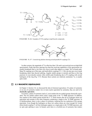
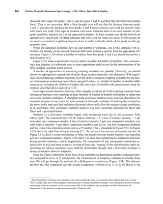
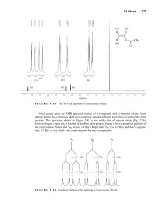
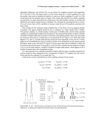
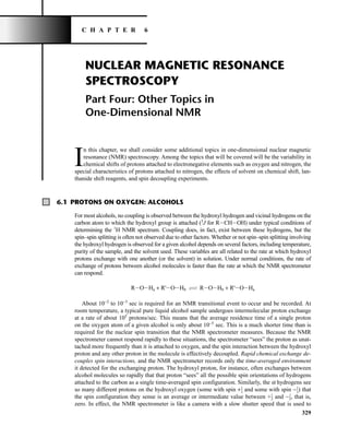
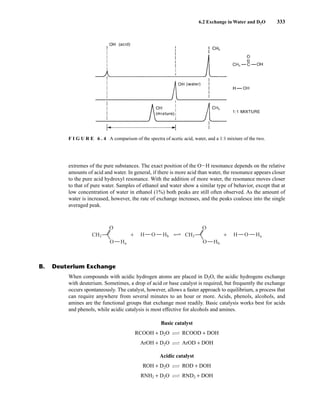
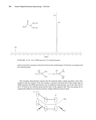
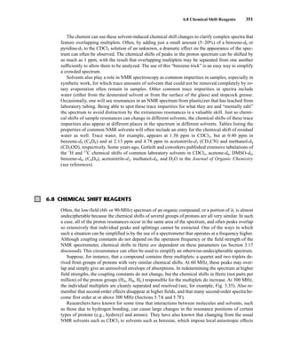
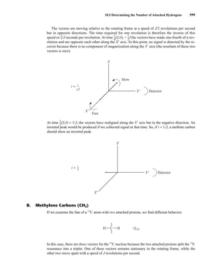
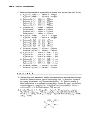
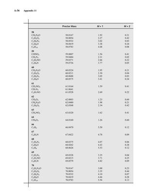
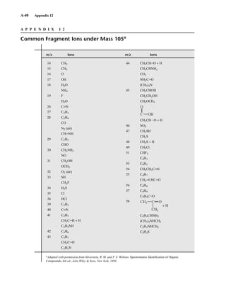
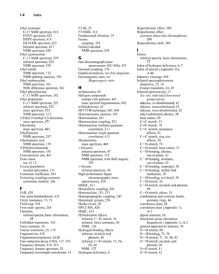
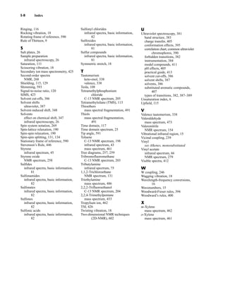
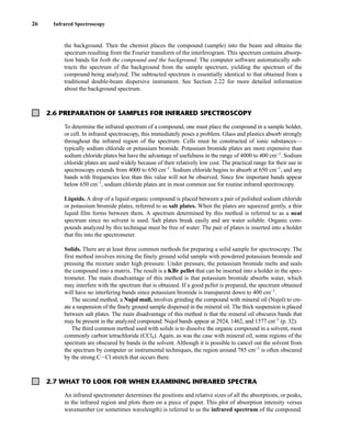
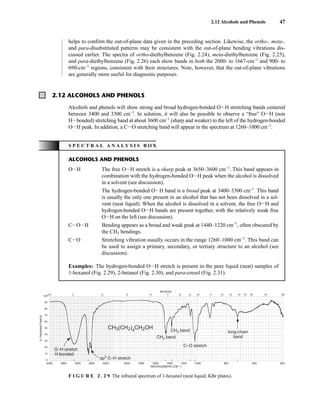
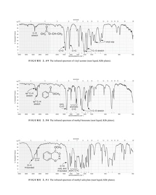
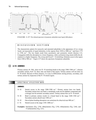
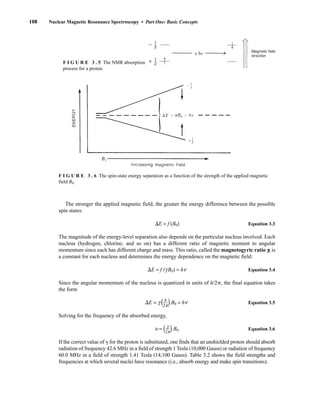
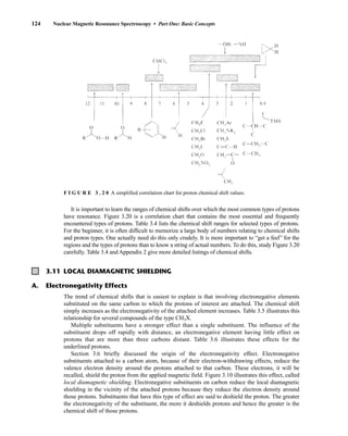
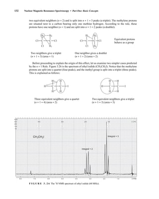
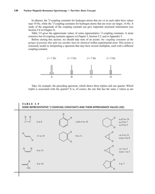
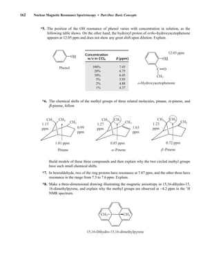
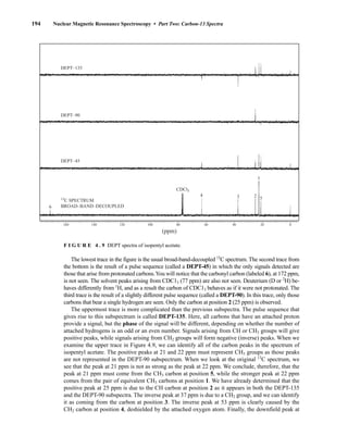
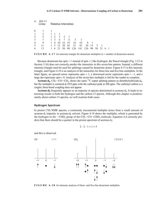
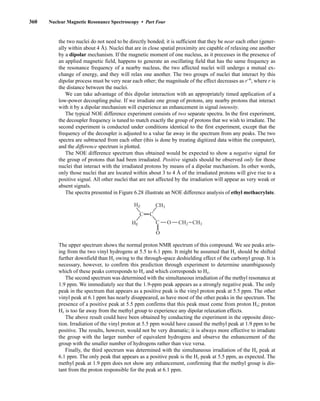
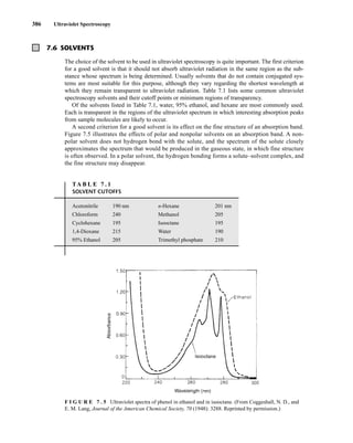
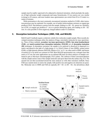
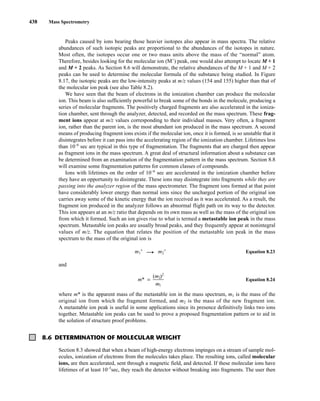
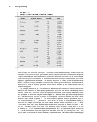
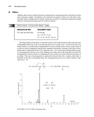
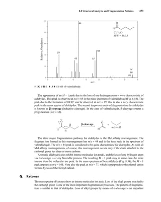
![354 Nuclear Magnetic Resonance Spectroscopy • Part Four
Today, most laboratories have access to high-field NMR spectrometers (operating at a 1
H
frequency of 300 MHz or greater), and simple chemical shift reagents as discussed above are infre-
quently used. Lanthanide complexes in which the organic ligand on the metal is optically active,
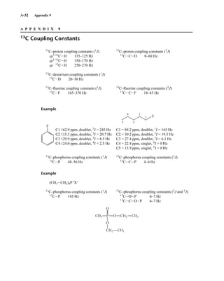
however, create a chiral shift reagent. One such reagent commonly used for this purpose is tris
[3-(heptafluoropropylhydroxymethylene)-d-camphorato] europium(III) [Eu(hfc)3]. When Eu(hfc)3
complexes to a chiral molecule, diastereomeric complexes are formed, which gives rise to different
chemical shifts for protons that were previously identical.
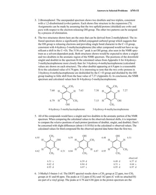
Tris[3-(heptafluoropropylhydroxymethylene)-d-camphorato] europium(III) [Eu(hfc)3]
O
O Eu
3
C3F7
CH3
H3C
H3C
6.9 CHIRAL RESOLVING AGENTS
A group attached to a stereocenter normally has the same chemical shift whether the stereogenic cen-
ter has R or S configuration. However, the group can be made diastereotopic in the NMR (have differ-
ent chemical shifts) when the racemic parent compound is treated with an optically pure chiral
resolving agent to produce diastereomers. In this case, the group is no longer present in two enan-
tiomers but in two different diastereomers, and its chemical shift is different in each environment.
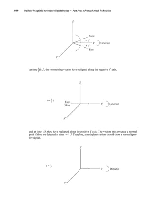
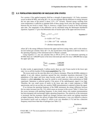
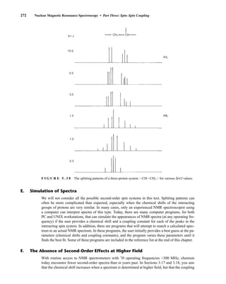
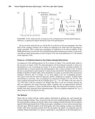
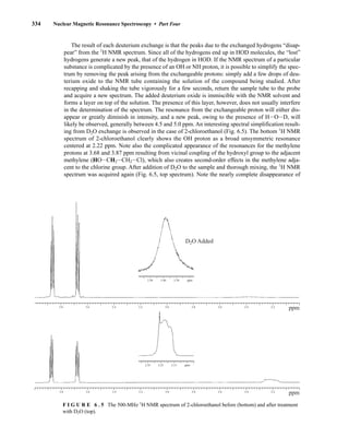
For instance, if a mixture containing both the R and S enantiomers of α-phenylethylamine is
mixed with an equimolar amount of optically pure (S)-(+)-O-acetylmandelic acid in an NMR tube
containing CDCl3, two diastereomeric salts form:
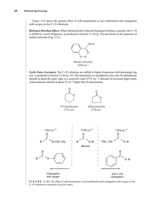
The methyl groups in the amine portion of the salts are attached to a stereocenter, S in one case and R
in the other. As a result, the methyl groups themselves are now diastereotopic, and they have different
chemical shifts. In this case, the R isomer is downfield, and the S isomer is upfield. Since the methyl
groups are adjacent to a methine (CH) group, they appear as doublets at approximately 1.1 and
1.2 ppm, respectively, in the NMR spectrum of the mixture (the exact chemical shifts vary slightly
with concentration) (Fig. 6.23).
These doublets may be integrated to determine the exact percentages of the R and S amines in the
mixture. In the example shown, the NMR spectrum was determined with a mixture made by dissolving
Ph
Ph
CH
CH3 CH COOH
OAc
NH2
Ph
+ Ph
CH
CH3 CH COO–
NH3
+
OAc
Ph
+ Ph
CH
CH3 CH COO–
NH3
+
OAc
(R/S) (S) (R) (S)
(S) (S)
α-Phenylethylamine
Diastereomers
+
S-(+)-O-acetyl-
mandelic acid
+
14782_06_Ch6_p329-380.pp3.qxd 2/6/08 8:15 AM Page 354](https://image.slidesharecdn.com/introductiontospectroscopy4ebypavia-240123161815-89f06477/85/Introduction-to-Spectroscopy-4e-by-Pavia-pdf-371-320.jpg)
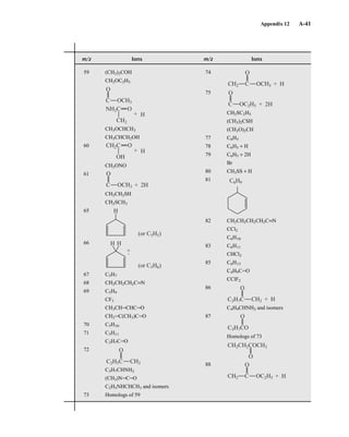
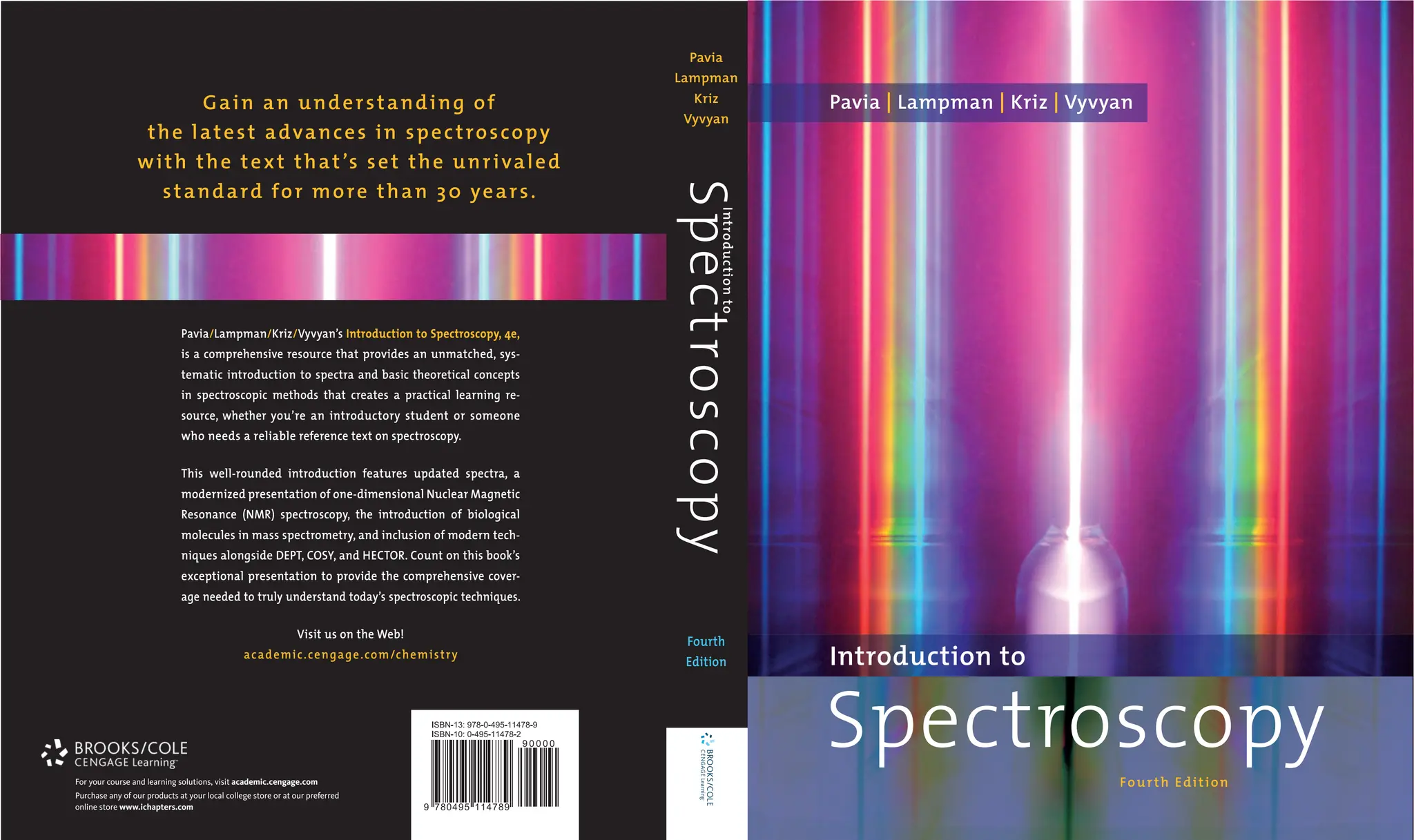
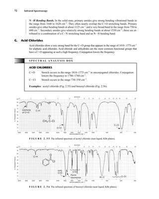
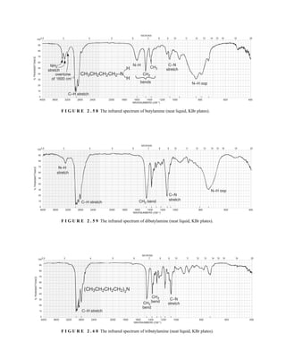
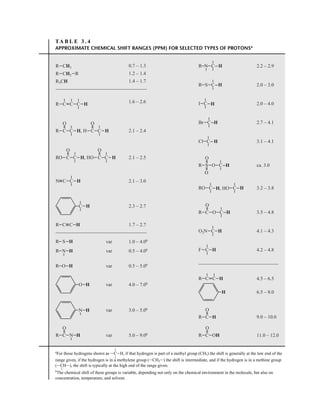
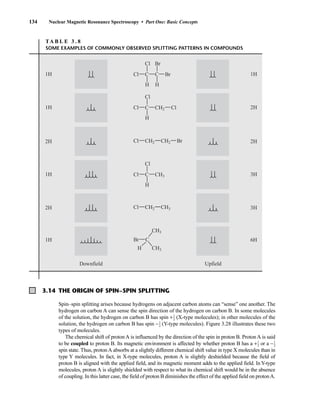
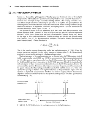
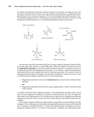
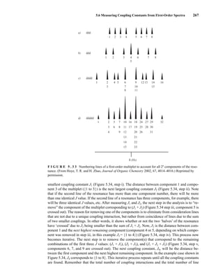
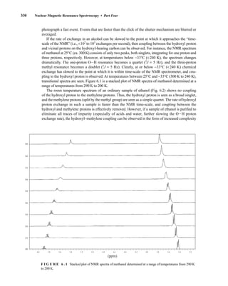
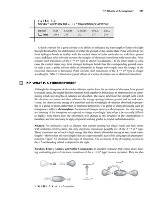
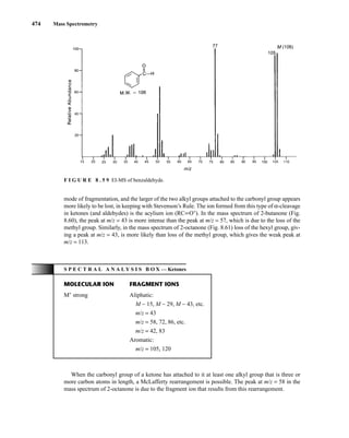
![6.9 Chiral Resolving Agents 355
equal quantities of unresolved (±)-α-phenylethylamine and a student’s resolved product, which con-
tained predominantly (S)-(−)-α-phenylethylamine.
Similarly, an optically pure amine can be used as a chiral resolving agent to analyze the optical
purity of a chiral carboxylic acid. For example, addition of optically pure (S)-(−)-α-phenylethylamine
to a CDCl3 solution of O-acetylmandelic acid will form diastereomeric salts as illustrated above. In
this case, one would look for the two doublets (one for each enantiomer) from the Ph−CH−OAc
methine between 5 and 6 ppm in the 1
H NMR spectrum.
When one needs to determine the optical purity of a compound that is not amenable to salt forma-
tion (i.e., not a carboxylic acid or amine), analysis by NMR becomes slightly more difficult. It is fre-
quently necessary to determine the enantiomeric excesses of chiral secondary alcohols, for example.
In these cases, derivatization of the alcohol through covalent attachment of an optically pure auxil-
iary provides the mixture of diastereomers for analysis. This requires reacting a (usually small, a few
milligrams) sample of sample alcohol with the optically pure derivatizing agent. Sometimes, purifi-
cation of the products is necessary. In the example shown below, a chiral secondary alcohol is reacted
with (S)-2-methoxyphenylacetic acid [(S)-MPA] using dicyclohexylcarbodiimide (DCC) to form di-
astereomeric esters. After workup, the 1
H NMR spectrum of product mixture is acquired, and the res-
onances from oxygenated methine (HCR1R2−O−Aux, there will be one signal for each diastereomer)
are integrated to determine the optical purity (enantiomeric excess) of the original alcohol sample.
Because the products are diastereomers, other methods of analysis (for example, gas chromatogra-
phy) could also be used for this purpose.
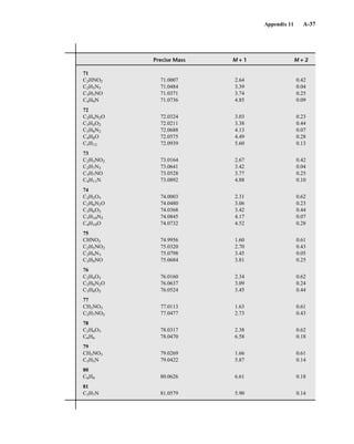
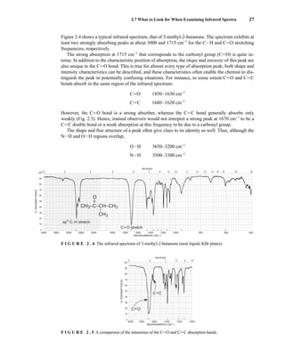
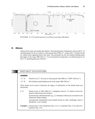
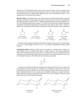
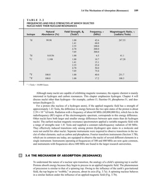
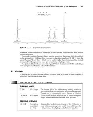
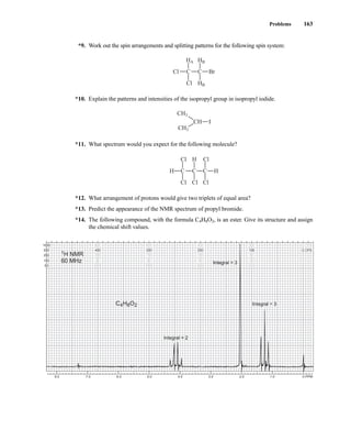
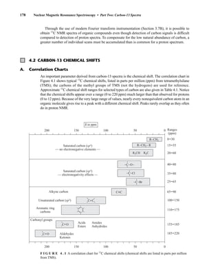
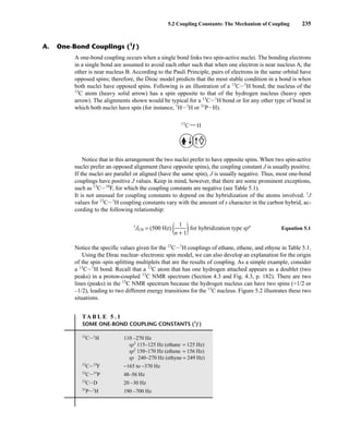
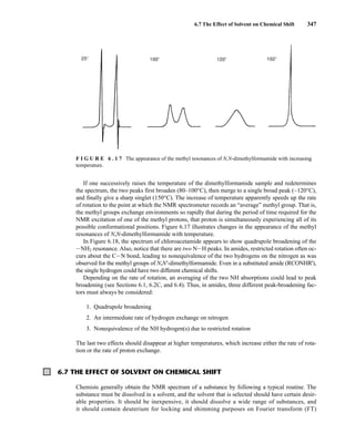
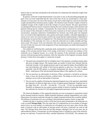
This process is illustrated in Figure 6.24 for 2-pentanol and α-methoxyphenylacetic acid (MPA).
To simplify the discussion, 1
H NMR spectra from two separate samples are shown. The ester formed
from (R)-2-pentanol and (R)-MPA produced the top spectrum in Figure 6.24, and the ester formed
from (R)-2-pentanol and (S)-MPA produced the bottom spectrum. Most diagnostic are the chemical
R S
1.25 1.20 1.15 1.10 1.05
PPM
295 mm
740 mm
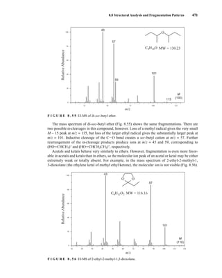
F I G U R E 6 . 2 3 The 300-MHz 1
H spectrum of a
50–50 mixture of (S)-α-phenylethylamine from a resolution
and unresolved (racemic) α-phenylethylamine in CDCl3
with the chiral resolving agent (S)-(+)-O-acetylmandelic
acid added.
14782_06_Ch6_p329-380.pp3.qxd 2/6/08 8:15 AM Page 355](https://image.slidesharecdn.com/introductiontospectroscopy4ebypavia-240123161815-89f06477/85/Introduction-to-Spectroscopy-4e-by-Pavia-pdf-372-320.jpg)
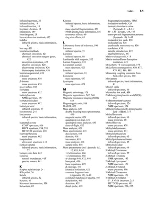
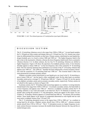
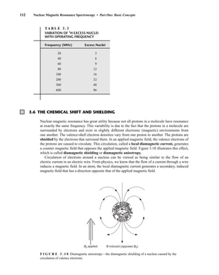
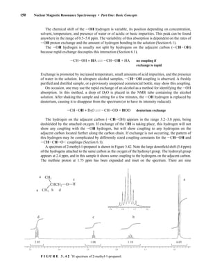
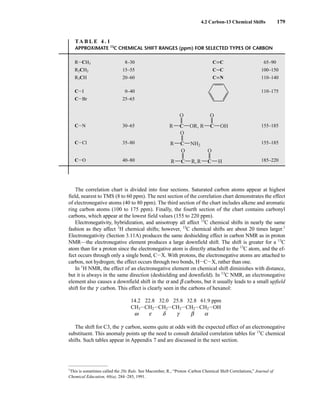
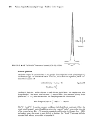
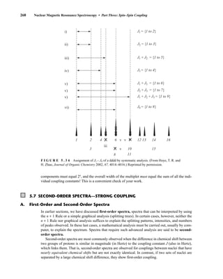
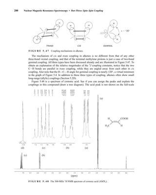
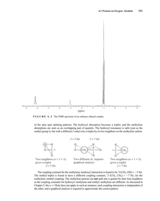
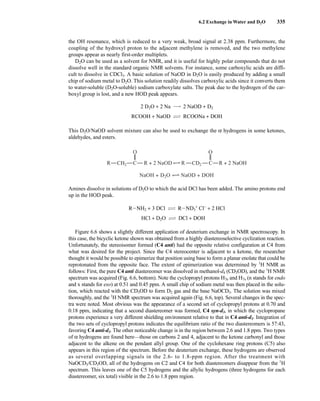
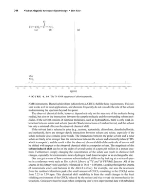
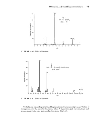
![6.10 Determining Absolute and Relative Configuration via NMR 357
to determine the absolute configuration of secondary alcohols by NMR analysis, and since that time
his method has been expanded and refined. In Mosher’s method, the alcohol is reacted separately
with each enantiomer of methoxytrifluoromethylphenylacetic acid (MTPA) or the corresponding
acid chloride (MTPA-Cl) (Fig. 6.25). Note that the carboxylic acid and the acid chloride have the
same three-dimensional arrangement of substituents on the stereogenic center but have opposite R/S
configurations as a result of a Cahn–Ingold–Prelog priority change in converting the −OH of the acid
to the –Cl of the acid chloride. This unfortunate circumstance has resulted in many instances of con-
fusion and incorrect stereochemical assignments.
After the two MTPA esters are prepared, the NMR spectrum (19
F, 1
H, and/or 13
C) of each deriv-
ative is acquired, and the chemical shifts of each resonance are compared. The chemical shift of
the resonances for the groups directly attached to the stereocenter in the spectrum of the (R) ester
is subtracted from the corresponding chemical shifts for those resonances in the spectrum of the
(S) ester [δ(S) − δ(R) = ΔδSR
]. The absolute configuration of the substrate is then deduced by inter-
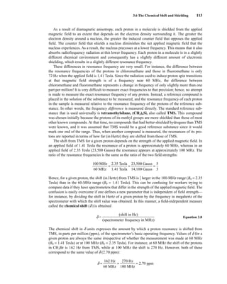
preting the signs of the Δδ values using certain empirical models for the most stable conformation
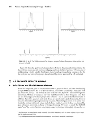
of the esters (Fig. 6.26). Based on his experiments, Mosher concluded that the CF3 group, Cα, the
carboxyl group of the ester, and the oxygenated methine (Cl') are all coplanar. This conformation
results in differential shielding of L1 and L2 by the phenyl group of the MTPA ester (see Section 3.12
for a discussion of shielding effects of aromatic rings). In the (R)-MTPA ester, L2 is shielded by
the phenyl group (Fig. 6.26a). The opposite is true in the (S)-MTPA ester—L1 is shielded by the
phenyl group (Fig. 6.26b). As a result, all the protons (or carbons) that are relatively shielded in
the (R)-MTPA ester will have a positive ΔδSR
value (L2 in Fig. 6.26c), and those not shielded by the
phenyl will have a negative ΔδSR
value (L1 in Fig. 6.26c). If the alcohol has the opposite configura-
tion, the shielding environments are reversed (Fig. 6.26d). Once the ΔδSR
values are determined for
the groups flanking the MTPA ester, one can use the structural models in Figure 6.26c and 6.26d to
assign L1 and L2 and thereby determine the absolute configuration of the original alcohol. In com-
mon practice, most researchers use the modified Mosher method, which involves examination of
the ΔδSR
values not just for the groups directly attached to the stereocenter in question, but to all
the protons (or carbons) in the compound. In this way, a representative sign of ΔδSR
for the sub-
stituents L1 and L2 can be determined, thus helping to prevent confusion that could arise from an
anomalous chemical shift.
O
X
H
X
OMe
Ph
OH
X Cl
HO
F3C
(R)-MTPA,
(S)-MTPACl,
L1
L2
or
(S)-MTPA
19F NMR Δδ (CF3)
1H,13C NMR Δδ (L1/L2)
(R)-MTPACl
or
O
O H
OMe
Ph
F3C
L1
L2
O
O H
MeO Ph
F3C
L1
L2
F I G U R E 6 . 2 5 Formation of Mosher ester derivatives (From Seco, J. M., E. Quinoa, and R. Riguera,
Chemical Reviews 104 (2004): 17–117.) Reprinted by permission.
14782_06_Ch6_p329-380.pp3.qxd 2/6/08 8:15 AM Page 357](https://image.slidesharecdn.com/introductiontospectroscopy4ebypavia-240123161815-89f06477/85/Introduction-to-Spectroscopy-4e-by-Pavia-pdf-374-320.jpg)
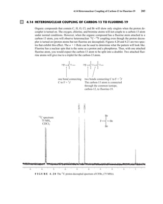
![358 Nuclear Magnetic Resonance Spectroscopy • Part Four
F I G U R E 6 . 2 6 Analysis of Mosher ester derivatives to determine. (From Seco, J. M., E. Quinoa, and
R. Riguera, Chemical Reviews 104 (2004): 17–117.)
H
(R)-MTPA
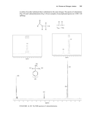
or
(S)-MTPACl
(S)-MTPA
or
(R)-MTPACl
•
•
•
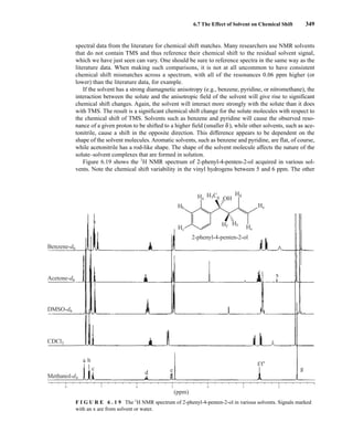
•
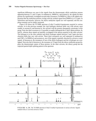
•
Ph
O
MeO
CF3
L1
L2 shielded
L2
L2
MTPAO ΔδSR0
ΔδSR0
Ph
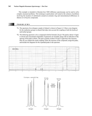
H
O
O
OMe
C(1')
F3C
L1
L2
Cα
a
c d
H
O L1
L2
Ph
O
MeO
F3C
Ph OMe
CF3
L1
L1 shielded
L2
b
L1
H
•
•
•
•
•
L1
MTPAO ΔδSR0
ΔδSR0
L2
O
The Mosher method can also be applied to β-chiral primary alcohols and α-chiral tertiary alco-
hols. Mosher amides can be prepared from chiral amines and analyzed in a similar fashion. A num-
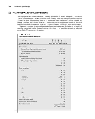
ber of other chiral derivatizing reagents for the determination of absolute configuration of alcohols,
amines, carboxylic acids, and sulfoxides have been developed over the years. In general, these chi-
ral auxiliaries all have three features in common: (1) a functional group that allows efficient cova-
lent attachment of the auxiliary to the substrate; (2) a polar or bulky group to fix the compound of
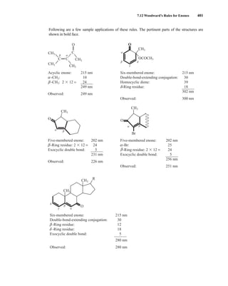
interest in a particular conformation; and (3) a group that is able to produce a significant anisotropic
effect in the dominant conformation that results in differential shielding in the two species (di-
astereomers) used in the determination.
Mosher originally used 19
F spectroscopy to determine absolute configuration of MTPA derivatives,
but today most researchers use 1
H NMR for this purpose. 19
F has the advantage of an uncrowded spec-
trum since the only fluorine signals are likely from the MTPA auxiliary itself. 1
H NMR is useful in most
circumstances, but overlap of resonances can still be a problem, even with a high-field spectrometer, if
ΔδSR
is small. 13
C NMR spectroscopy has the advantage of a wider chemical shift range and therefore
less likelihood of resonance overlap. Furthermore, 13
C NMR provides useful information even when
one or more of the substituents on the stereocenter have no protons. The low sensitivity of 13
C, however,
presents a limitation if only minute quantities of the substrates are available.
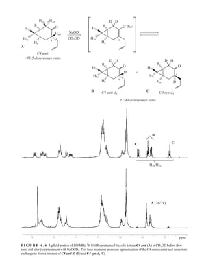
B. Determining Relative Configuration
In Chapter 5, we saw many instances when 1
H−1
H coupling constants could be used to assign relative
configuration, especially when the conformation of the compound can be inferred. We will not expand
on that discussion here. For some classes of compounds, simple 13
C NMR spectroscopy can be used
very reliably to assign relative stereochemical configuration. One of the most reliable examples is the
[l3
C]acetonide method for determining relative configuration of acyclic 1,3-diols. The conformational
preferences for 2,2-dimethyl-l,3-dioxolanes (acetone ketals, acetonides) were already well known by
1990, when Rychnovsky correlated the l3
C chemical shifts of acetonide methyl groups to stereochemical
configuration. Acetonides of syn-1,3-diols adopted a chair conformation in which one methyl group of
the acetonide is in an axial position and the other methyl group is in an equatorial position. The methyl
group in the more shielded axial position has a chemical shift of ~19 ppm in the l3
C NMR spectrum and
the less-shielded methyl group in the equatorial position appears at ~30 ppm (Fig. 6.27). Conversely,
14782_06_Ch6_p329-380.pp3.qxd 2/6/08 8:15 AM Page 358](https://image.slidesharecdn.com/introductiontospectroscopy4ebypavia-240123161815-89f06477/85/Introduction-to-Spectroscopy-4e-by-Pavia-pdf-375-320.jpg)
![6.11 Nuclear Overhauser Effect Difference Spectra 359
6.11 NUCLEAR OVERHAUSER EFFECT DIFFERENCE SPECTRA
the acetonide derivatives of anti-1,3-diols exist in a twist boat conformation to alleviate steric repul-
sions in the chair conformations. In the anti-1,3-diol acetonides, the two methyl groups both appear at
~25 ppm in the l3
C NMR spectrum. The chemical shift of the acetal carbon also correlates well to stere-
ochemical configuration, with the acetal carbon of syn-1,3-diol acetonides appearing at 98.5 ppm and
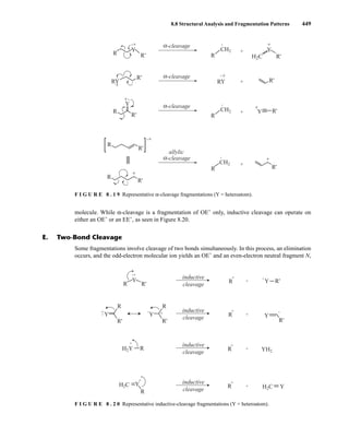
that of the anti-1,3-diol acetonide appearing at 100.6 ppm in the 13
C NMR spectrum.
Analysis of literature 13
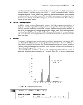
C NMR data for hundreds of 1,3-diol acetonides have proven this method
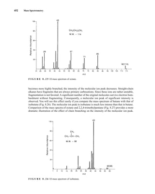
reliable. Only a few types of substituents (R1 and/or R2) are problematic. The chemical shift correla-
tions shown in Figure 6.27 only become unreliable when the substituents in the 4 and/or 6 position of
the dioxolane ring are an sp-hybridized carbon (alkyne or nitrile). Use of the acetal carbon chemical
shift correlation is not quite as reliable, but of the hundreds of acetonides examined, fewer than 10%
of syn-l,3-diol acetonides and 5% of anti-1,3-diol acetonides would be misassigned based on the
chemical shift of the acetal carbon alone—and practially none will be misassigned if the acetal
chemical shift is considered in conjunction with the acetonide methyl chemical shifts. The only
drawbacks to this method is that the acetonide derivatives must be prepared from the diol substrates,
but this is easily accomplished with a mixture of acetone, 2,2-dimethoxypropane, and pyridinium/
p-toluenesulfonate (PPTS). When only a small amount of sample is available, 13
C-enriched acetone can
be used to prepare the acetonides. The [l3
C]acetonide method is also readily applied to complex
natural products containing several different 1,3-diols.
syn-1, 3-diol acetonide
anti-1, 3-diol acetonide Twist-boat
Chair
R1
H
H
R2
O
O
CH3
CH3
30.0 ppm
98.5 ppm
19.6 ppm
R1
O O
R2
2
6
4
R1
O O
R2
2
6
4
O
O
H
H
R2
R1
CH3
CH3
24.6 ppm
24.6 ppm
100.6 ppm
F I G U R E 6 . 2 7 13
C NMR chemical shift correlations for 1,3-diol acetonides. (From Rychnovsky, S. D.,
B. N. Rogers, and T. I. Richardson, Accounts of Chemical Research 31 (1998): 9–17.)
In many cases of interpretation of NMR spectra, it would be helpful to be able to distinguish pro-
tons by their spatial location within a molecule. For example, for alkenes it would be useful to de-
termine whether two groups are cis to each other or whether they represent a trans isomer. In
bicyclic molecules, the chemist may wish to know whether a substituent is in an exo or in an endo
position. Many of these types of problems cannot be solved by an analysis of chemical shift or by
examination of spin–spin splitting effects.
A handy method for solving these types of problems is nuclear Overhauser effect (NOE) differ-
ence spectroscopy. This technique is based on the same phenomenon that gives rise to the nuclear
Overhauser effect (Section 4.5), except that it uses homonuclear, rather than a heteronuclear, de-
coupling. In the discussion of the nuclear Overhauser effect, attention was focused on the case in
which a hydrogen atom was directly bonded to a 13
C atom, and the hydrogen nucleus was saturated
by a broadband signal. In fact, however, for two nuclei to interact via the nuclear Overhauser effect,
14782_06_Ch6_p329-380.pp3.qxd 2/6/08 8:15 AM Page 359](https://image.slidesharecdn.com/introductiontospectroscopy4ebypavia-240123161815-89f06477/85/Introduction-to-Spectroscopy-4e-by-Pavia-pdf-376-320.jpg)
![380 Nuclear Magnetic Resonance Spectroscopy • Part Four
20. In Problem 11, calculations proved to be a good way of assigning structures to the spectra of
some aromatic amines. Describe an experimental way of differentiating between the
following amines:
NH2 NH2
CH3
NO2
NO2
CH3
*21. At room temperature, the NMR spectrum of cyclohexane shows only a single resonance peak.
As the temperature of the sample is lowered, the sharp single peak broadens until at −66.7°C it
begins to split into two peaks, both broad. As the temperature is lowered further to −100°C,
each of the two broad bands begins to give a splitting pattern of its own. Explain the origin of
these two families of bands.
*22. In cis-1-bromo-4-tert-butylcyclohexane, the proton on carbon-4 is found to give resonance at
4.33 ppm. In the trans isomer, the resonance of the C4 hydrogen is at 3.63 ppm. Explain why
these compounds should have different chemical shift values for the C4 hydrogen. Can you
explain the fact that this difference is not seen in the 4-bromomethylcyclohexanes except at
very low temperature?
Crews, P., J. Rodriguez, and M. Jaspars, Organic Structure
Analysis, Oxford University Press, New York, 1998.
Friebolin, H., Basic One- and Two-Dimensional NMR Spec-
troscopy, 3rd ed., Wiley-VCH, New York, 1998.
Gotlieb, H. E., V. Kotlyar, and A. Nudelman. “NMR Chemi-
cal Shifts of Common Laboratory Solvents as Trace Im-
purities,” Journal of Organic Chemistry 62 (1997):
7512–7515.
Gunther, H., NMR Spectroscopy, 2nd ed., John Wiley and
Sons, New York, 1995.
Jackman, L. M., and S. Sternhell, Applications of Nuclear
Magnetic Resonance Spectroscopy in Organic Chem-
istry, 2nd ed., Pergamon Press, London, 1969.
Lambert, J. B., H. F. Shurvell, D. A. Lightner, and R. G.
Cooks, Organic Structural Spectroscopy, Prentice Hall,
Upper Saddle River, NJ, 1998.
Macomber, R. S., NMR Spectroscopy—Essential Theory
and Practice, College Outline Series, Harcourt, Brace
Jovanovich, New York, 1988.
Macomber, R. S., A Complete Introduction to Modern NMR
Spectroscopy, John Wiley and Sons, New York, 1997.
Pople, J. A., W. C. Schneider, and H. J. Bernstein, High Res-
olution Nuclear Magnetic Resonance, McGraw–Hill,
New York, 1969.
Pouchert, C. and J. Behnke, Aldrich Library of 13
C and 1
H FT-
NMR Spectra,Aldrich Chemical Co., Milwaukee, WI, 1993.
R E F E R E N C E S
Rothchild, R., “NMR Methods for Determination of Enan-
tiomeric Excess,” Enantiomer 5 (2000): 457–471.
Rychnovsky, S. D., B. N. Rogers, and G. Yang, “Analysis of
Two Carbon-13 NMR Correlations for Determining the
Stereochemistry of 1,3-Diol Acetonides,” Journal of Or-
ganic Chemistry 58 (1993): 3511–3515.
Rychnovsky, S. D., B. N. Rogers, and T. I. Richardson,
“Configurational Assignment of Polyene Macrolide An-
tibiotics Using the [13
C] Acetonide Analysis,” Accounts
of Chemical Research 31 (1998): 9–17.
Sanders, J. K. M., and B. K. Hunter, Modern NMR Spec-
troscopy—A Guide for Chemists, 2nd ed., Oxford
University Press, Oxford, England, 1993.
Seco, J. M., E. Quinoa, and R. Riguera, “The Assignment of
Absolute Configuration by NMR,” Chemical Reviews
104 (2004): 17–117 and references therein.
Silverstein, R. M., F. X. Webster, and D. J. Kiemle, Spectro-
metric Identification of Organic Compounds, 7th ed.,
John Wiley and Sons, New York, 2005.
Yoder, C. H., and C. D. Schaeffer, Introduction to Multinu-
clear NMR, Benjamin–Cummings, Menlo Park, CA,
1987.
In addition to these references, also consult textbook refer-
ences, compilations of spectra, computer programs, and
NMR-related Internet addresses cited at the end of
Chapter 5.
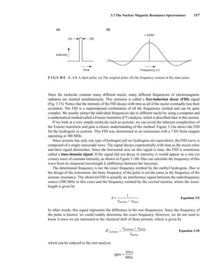
14782_06_Ch6_p329-380.pp3.qxd 2/6/08 8:15 AM Page 380](https://image.slidesharecdn.com/introductiontospectroscopy4ebypavia-240123161815-89f06477/85/Introduction-to-Spectroscopy-4e-by-Pavia-pdf-397-320.jpg)
![381
C H A P T E R 7
ULTRAVIOLET SPECTROSCOPY
M
ost organic molecules and functional groups are transparent in the portions of the electro-
magnetic spectrum that we call the ultraviolet (UV) and visible (VIS) regions—that is, the
regions where wavelengths range from 190 nm to 800 nm. Consequently, absorption spec-
troscopy is of limited utility in this range of wavelengths. However, in some cases we can derive use-
ful information from these regions of the spectrum. That information, when combined with the detail
provided by infrared and nuclear magnetic resonance (NMR) spectra, can lead to valuable structural
proposals.
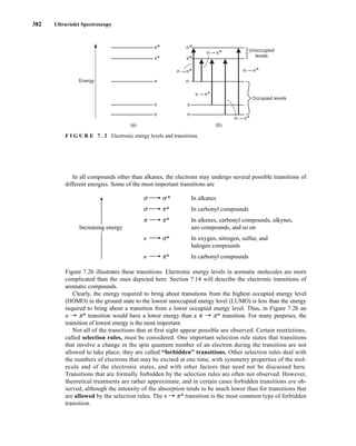
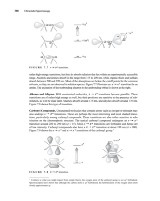
7.1 THE NATURE OF ELECTRONIC EXCITATIONS
When continuous radiation passes through a transparent material, a portion of the radiation may be
absorbed. If that occurs, the residual radiation, when it is passed through a prism, yields a spectrum
with gaps in it, called an absorption spectrum. As a result of energy absorption, atoms or mole-
cules pass from a state of low energy (the initial, or ground state) to a state of higher energy (the
excited state). Figure 7.1 depicts this excitation process, which is quantized. The electromagnetic
radiation that is absorbed has energy exactly equal to the energy difference between the excited and
ground states.
In the case of ultraviolet and visible spectroscopy, the transitions that result in the absorption of
electromagnetic radiation in this region of the spectrum are transitions between electronic energy
levels. As a molecule absorbs energy, an electron is promoted from an occupied orbital to an
unoccupied orbital of greater potential energy. Generally, the most probable transition is from the
highest occupied molecular orbital (HOMO) to the lowest unoccupied molecular orbital
(LUMO). The energy differences between electronic levels in most molecules vary from 125 to
650 kJ/mole (kilojoules per mole).
For most molecules, the lowest-energy occupied molecular orbitals are the s orbitals, which
correspond to s bonds. The p orbitals lie at somewhat higher energy levels, and orbitals that hold
unshared pairs, the nonbonding (n) orbitals, lie at even higher energies. The unoccupied, or
antibonding orbitals (p * and s *), are the orbitals of highest energy. Figure 7.2a shows a typical
progression of electronic energy levels.
E(excited)
ΔE = [E(excited) – E(ground)]
= hυ
E(ground)
F I G U R E 7 . 1 The excitation process.
14782_07_Ch7_p381-417.pp2.qxd 2/2/08 1:22 AM Page 381](https://image.slidesharecdn.com/introductiontospectroscopy4ebypavia-240123161815-89f06477/85/Introduction-to-Spectroscopy-4e-by-Pavia-pdf-398-320.jpg)
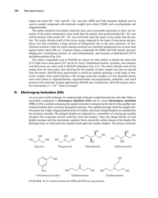
![422 Mass Spectrometry
Reagent Gas
Proton
Affinity
(kcal/mole)
Reagent
Ion(s) Analyte Ion(s) Comments
H2 101 H3
+
(M + H)+ Produces significant fragmentation
CH4 132 CH5
+
, C2H5
+
(M + H)+
, (M + C2H5)+ Less fragmentation than H2, can form
adducts
NH3 204 NH4
+
(M + H)+
, (M + NH4)+ Selective ionization, little fragmenta-
tion, some adduct formation
(CH3)3CH 196 (CH3)3C+
(M + H)+
,
[M + C(CH3)3)]+
Mild, selective protonation, little
fragmentation
CH3OH 182 CH3OH2
+
(M + H)+ Degree of fragmentation observed
between that of methane and isobutane
CH3CN 188 CH3CNH+
(M + H)+ Degree of fragmentation observed
between that of methane and isobutane
TA B L E 8 . 1
SUMMARY OF CHEMICAL IONIZATION (CI) REAGENT GASES
The situation is very similar for CI with ammonia as reagent gas (Equations 8.7–8.9):
NH3 + e−
→ ΝΗ3
• +
+ 2e−
Equation 8.7
NH3
• +
+ NH3 → ΝΗ4
+
+ • NH2 Equation 8.8
M + NH4
+
→ (Μ + Η)+
+ NH3 Equation 8.9
Using isobutane as reagent gas produces tert-butyl cations (Equations 8.10 and 8.11), which readily
protonate basic sites on the sample molecule (Equation 8.12). Adduct formation is also possible
using isobutane in CI-MS (Equation 8.l3).
(CH3)3CH + e−
→ (CH3)3CH• +
+ 2e−
Equation 8.10
(CH3)3CH• +
→ (CH3)3C+
+ H• Equation 8.11
M + (CH3)3C+
→ (Μ + H)+
+ (CH3)2CJCH2 Equation 8.12
M + (CH3)3C+
→ [Μ + C(CH3)3]+
Equation 8.13
Varying the reagent gas in CI-MS allows one to vary the selectivity of the ionization and degree of
ion fragmentation. The choice of reagent gas should be made carefully to best match the proton
affinity of the reagent gas with that of the sample to ensure efficient ionization of the sample without
excessive fragmentation. The greater the difference between the proton affinity of the sample and
that of the reagent gas, the more energy that is transferred to the sample during ionization. The excess
energy produces an analyte ion in a highly excited vibrational state. If enough excess kinetic energy
is transferred, the sample ion will fragment through the cleavage of covalent bonds. Therefore, using
a reagent gas with a proton affinity matched closely to that of the sample will result in a greater num-
ber of intact molecular ions and smaller number of fragment ions. It is unlikely, of course, that one
knows the precise proton affinity of the sample, but one can estimate the value by looking at tables of
values determined for simple compounds with functional groups similar to the sample in question.
A summary of common CI reagent gases and their ions/properties is presented in Table 8.l.
As one can see from Figure 8.3, CI-MS of lavandulyl acetate (MW 196) gives mass spectra with
very different appearances depending on the regent gas used to ionize the sample. In the top spectrum,
14782_08_Ch8_p418-519.pp3.qxd 2/6/08 3:06 PM Page 422](https://image.slidesharecdn.com/introductiontospectroscopy4ebypavia-240123161815-89f06477/85/Introduction-to-Spectroscopy-4e-by-Pavia-pdf-439-320.jpg)
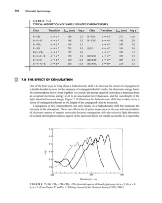
![8.3 Ionization Methods 423
the protonated molecular ion of lavandulyl acetate [(M + H)+
, m/z = 197] is barely visible, and the
largest peak in the spectrum belongs to the fragment at m/z = 137. In the middle spectrum, acquired
using isobutane as reagent gas, the protonated molecular ion at m/z = 197 is much more prominent,
and there is less overall fragmentation. Fragmentation is still significant in this case, though, as the ion
at m/z = 137 is still the most abundant in the spectrum. Finally, when lavandulyl acetate is ionized
using ammonia, the protonated molecular ion is the most abundant ion (the base peak), and almost no
fragmentation is observed. Note the presence of an adduct ion [(M + NH4)+
, m/z = 214] present in this
spectrum.
As a practical note, spectra acquired under CI conditions are usually acquired over a mass range
above the m/z of the reagent gas ions. The ionized reagent gas is also detected by the spectrometer,
and because the reagent gas is present in great excess relative to the sample, its ions would dominate
the spectrum. Thus, CI (methane) spectra are typically acquired above m/z = 50 (CH5
+
is m/z = 17,
F I G U R E 8 . 3 Comparison of CI-MS data of lavandulyl acetate using methane (top), isobutane
(middle), and ammonia (bottom) as reagent gases. (From McLafferty, F. W. and F. Tureček, Interpretation of
Mass Spectra, 4th
ed., University Science Books, Mill Valley, CA, 1993. Reprinted with permission.)
100
50
100
95
m/z
81
Relative
Abundance
137
109
121 197 MH+
197 MH+
120 140 160 180 200 220
95
m/z
81
50
100
Relative
Abundance
137
109 123 179
100 120 140 160 180 200 220
93
m/z
50
100
Relative
Abundance
137
154
121
197
214 M + NH4
+
100 120 140 160 180 200 220
137
HO+
C
O
14782_08_Ch8_p418-519.pp3.qxd 2/6/08 3:06 PM Page 423](https://image.slidesharecdn.com/introductiontospectroscopy4ebypavia-240123161815-89f06477/85/Introduction-to-Spectroscopy-4e-by-Pavia-pdf-440-320.jpg)
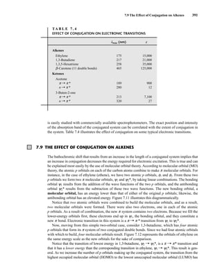
![424 Mass Spectrometry
F I G U R E 8 . 4 MS of butyl methacrylate acquired under EI (top) and CI (methane, middle; isobutane,
bottom) conditions. (From DeHoffmann, E. and V. Stroobant, Mass Spectrometry: Principles and
Applications, 2nd ed., John Wiley and Sons, New York, 1999. Reprinted with permission.)
56
69
87
87
69
61 81 100
115
127
143
82 100
40
6000
8000
4000
2000
4500
3000
1500
1200
900
600
300
m/z
m/z
m/z
60
73 87
81 97 113
143
60 80 100 120 140 160 180
60 80 100 120 140 160 180
60 80 100 120 140 160 180
O
O
Intensity
(arbitrary
units)
Intensity
(arbitrary
units)
Intensity
(arbitrary
units)
of course, but C2H5
+
[m/z = 29] and C3H5
+
[m/z = 41] are also present), and CI (isobutane) spectra
are typically acquired above m/z = 60 or 70.
The main advantage of CI-MS is the selective production of intact quasi-molecular ions
[(M + H)+
]. Figure 8.4 shows the mass spectrum of butyl methacrylate acquired under different ion-
ization conditions. The molecular ion (m/z = 142) is barely visible in the EI-MS, but the
(M + H)+
ion (m/z = 143) is prominent in the CI-MS spectra. The CI-MS acquired using isobutane
has much less fragmentation than the CI-MS acquired using methane as the reagent gas. Other
advantages to CI-MS include inexpensive and robust hardware. Like in EI-MS, however, the
14782_08_Ch8_p418-519.pp3.qxd 2/6/08 3:06 PM Page 424](https://image.slidesharecdn.com/introductiontospectroscopy4ebypavia-240123161815-89f06477/85/Introduction-to-Spectroscopy-4e-by-Pavia-pdf-441-320.jpg)
![428 Mass Spectrometry
The charges of the ions generated using ESI do not necessarily reflect the charge state of the
sample in solution. The charge transferred to the sample molecules (usually in the form of protons)
arises from a combination of charge concentration in the droplets during evaporation of the aerosol
and electrochemical processes stemming from the electrostatic potential of the capillary.
The sample ions may bear a single charge or multiple charges. Figure 8.9 shows the ESI-MS of
lysozyme from chicken egg white in the absence and presence of dithiothreitol. In the first spec-
trum, ions are observed representing protein molecules bearing 10+
, 11+
, 12+
, and 13+
charges. The
latter spectrum shows even more highly charged ions—including a peak from protein bearing a
20+
charge. The formation of multiply charged ions is particularly useful in the MS analysis of
proteins. Typical proteins can carry many protons due to the presence of basic amino acid side
chains, resulting in peaks at m/z = 600–2000 for proteins with a molecular weight that approaches
200,000 amu.
The data shown in Figure 8.9 can be used to calculate the molecular mass for lysozyme. The mass
is calculated by multiplying the charge on the lysozyme by the m/z value shown on the chro-
matogram. For example:
(10)(1432) 5 14,320 AMU
(12)(1193) 5 14,316
(15)(955) 5 14,325
Thus, the molecular mass of lysozyme is about 14,320 AMU.
100
0
600 800 1000 1200 1600
1400 m/z
Relative
Abundance
[%]
with 1,4-dithiothreitol
hen egg white lysozyme
Mr = 14,306
1023
1101
1193
1302
1023 1001
898
843
796
20+
10+
1433
15+
955
1193
12+
1302
10+
1432
a
b
F I G U R E 8 . 9 ESI-MS of proteins. Chicken egg white lysozyme in the absence (top) and presence
(middle) of dithiothreitol. (From Gross, J. H., Mass Spectrometry: A Textbook, Spinger, Berlin, 2004.
Reprinted with permission.)
14782_08_Ch8_p418-519.pp3.qxd 2/6/08 3:06 PM Page 428](https://image.slidesharecdn.com/introductiontospectroscopy4ebypavia-240123161815-89f06477/85/Introduction-to-Spectroscopy-4e-by-Pavia-pdf-445-320.jpg)
![444 Mass Spectrometry
relative to the intensity of the molecular ion peak are unique. Thus, the isotope ratio method can be
used to establish the molecular formula of a compound. Examination of the intensity of the M + 2
peak is also useful for obtaining information about elements that may be present in the molecular for-
mula. An unusually intense M + 2 peak can indicate that sulfur or silicon is present in the unknown
substance. The relative abundances of 33
S and 34
S are 0.78 and 4.40, respectively, and the relative
abundance of 30
Si is 3.35. A trained chemist knows that a larger-than-normal M + 2 peak can be the
first hint that sulfur or silicon is present. Chlorine and bromine also have important M + 2 isotopes,
and they are discussed separately below.
Tables of possible combinations of carbon, hydrogen, oxygen, and nitrogen and intensity ratios
for the M + 1 and M + 2 peaks for each combination have been developed. An example of this sort
of table is found in Appendix 11. More extensive tables of intensity ratios for the M + 1 and M + 2
peaks may be found in specialized books on interpreting mass spectra. Accurate calculation of
the relative intensities of isotope peaks in a molecular ion cluster for compounds containing several
elements with isotopes is time consuming to do by hand as it requires polynomial expansions.
Fortunately, many websites dealing with mass spectrometry have isotope calculators that make this
a trivial task. Some of these sites may be found in the references at the end of this chapter.
For compounds containing only C, H, N, O, F, Si, P, and S, the relative intensities of M + 1 and
M + 2 peaks can be estimated quickly using simplified calculations. The formula to calculate the
M + 1 peak intensity (relative to M1
= 100) for a given formula is found in Equation 8.25.
Similarly, the intensity of an M + 2 peak intensity (relative to M1
= 100) may be found by using
Equation 8.26.
= (number of C × 1.1) + (number of H × 0.015) + (number of N × 0.37) +
(number of O × 0.04) + (number of S × 0.8) + (number of Si × 5.1) Equation 8.25
= + (number of O × 0.2) + (number of S × 4.4) + (number of Si × 3.4)
Equation 8.26
(number of C × 1.1)2
200
[M + 2]
[M + 1]
TA B L E 8 . 6
ISOTOPE RATIOS FOR PROPENE AND DIAZOMETHANE
Relative Intensities
Compound Molecular Mass M M ⴙ 1 M ⴙ 2
C3H6 42 100 3.34 0.05
CH2N2 42 100 1.87 0.01
TA B L E 8 . 7
ISOTOPE RATIOS FOR CO, N2, AND C2H4
Relative Intensities
Compound Molecular Mass M M ⴙ 1 M ⴙ 2
CO 28 100 1.12 0.2
N2 28 100 0.76
C2H4 28 100 2.23 0.01
14782_08_Ch8_p418-519.pp3.qxd 2/6/08 3:06 PM Page 444](https://image.slidesharecdn.com/introductiontospectroscopy4ebypavia-240123161815-89f06477/85/Introduction-to-Spectroscopy-4e-by-Pavia-pdf-461-320.jpg)
![450 Mass Spectrometry
usually a stable small molecule of some type: H2O, a hydrogen halide, or an alkene. Some examples
of two-bond cleavages of this type are shown in Figure 8.21.
Unsaturated six-membered rings can undergo a retro Diels–Alder fragmentation to produce the rad-
ical cation of a diene and a neutral alkene—the hypothetical precursors to the cyclohexene derivative
if it had been prepared in the forward direction via the [4π + 2π] diene + dienophile cycloaddition
known to every organic chemist as the Diels–Alder reaction. A schematic representation of the retro
Diels–Alder fragmentation is shown in Figure 8.22 Note that the unpaired electron and charge
remain with the diene fragment according to Stevenson’s Rule.
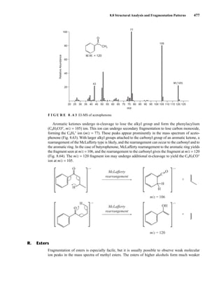
Another very common fragmentation that can occur with many substrates is the McLafferty
rearrangement (Fig. 8.23). This fragmentation was first described by Fred McLafferty in 1956
and is one of the most predictable fragmentations, next to the simple α-cleavage. In the
McLafferty rearrangement, a hydrogen atom on a carbon 3 atom away from the radical cation of
an alkene, arene, carbonyl, or imine (a so-called γ-hydrogen) is transferred to the charge site via a
six-membered transition state, with concurrent cleavage of the sigma bond between the α and β
positions of the tether. This forms a new radical cation and an alkene with a π bond between what
R
H2C CH2
X = OH, halide
n = 0, 1, 2, 3
R
H H
X X
n
n
n
n
R'
R R'
R R'
R'
+
+
•
+
•
+
•
•
elimination
elimination
F I G U R E 8 . 2 1 Common two-bond fragmentations (X = heteroatom).
+
McLafferty
rearrangement R
• +
Y
H
Z
Z, Y = C, N, O
R
α
β
γ
• +
Y
H
Z
F I G U R E 8 . 2 3 The McLafferty rearrangement.
+
retro
Diels–Alder
• +
R
R′
R
• +
R′
F I G U R E 8 . 2 2 A retro Diels–Alder fragmentation.
F. Retro Diels-Alder Cleavage
G. McLafferty Rearrangements
14782_08_Ch8_p418-519.pp3.qxd 2/6/08 3:06 PM Page 450](https://image.slidesharecdn.com/introductiontospectroscopy4ebypavia-240123161815-89f06477/85/Introduction-to-Spectroscopy-4e-by-Pavia-pdf-467-320.jpg)
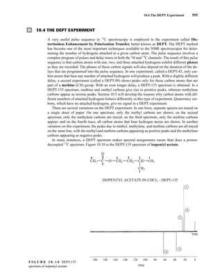
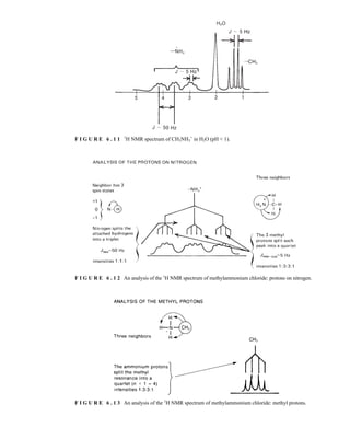
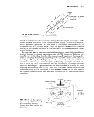
![454 Mass Spectrometry
F I G U R E 8 . 2 8 EI mass spectrum of cyclopentane.
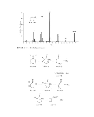
Cycloalkanes generally form strong molecular ion peaks. Fragmentation via the loss of a molecule of
ethene (M − 28) is common. The typical mass spectrum for a cycloalkane shows a relatively intense
molecular ion peak. Fragmentation of ring compounds requires the cleavage of two carbon–carbon
bonds, which is a more difficult process than cleavage of one such bond. Therefore, a larger proportion
of cycloalkane molecules than of acyclic alkane molecules survives electron bombardment without
undergoing fragmentation. In the mass spectra of cyclopentane (Fig. 8.28) and methylcyclopentane
(Fig. 8.29), strong molecular ion peaks can be observed.
The fragmentation patterns of cycloalkanes may show mass clusters arranged in a homologous
series, as in the alkanes. However, the most significant mode of cleavage of the cycloalkanes involves
the loss of a molecule of ethene (H2CJCH2), either from the parent molecule or from intermediate
OE+
. The peak at m/z = 42 in cyclopentane and the peak at m/z = 56 in methylcyclopentane result
from the loss of ethene from the parent molecule. Each of these fragment peaks is the most intense in
the mass spectrum. When the cycloalkane bears a side chain, loss of that side chain is a favorable
mode of fragmentation. The fragment peak at m/z = 69 in the mass spectrum of methylcyclopentane
is due to the loss of the CH3 side chain, which results in a secondary carbocation.
J. Cycloalkanes
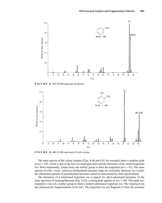
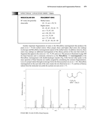
S P E C T R A L A N A L Y S I S B O X — Cycloalkanes
MOLECULAR ION FRAGMENT IONS
Strong M+
M − 28
A series of peaks: M − 15, M − 29, M − 43, M − 57, etc.
Applying these pieces of information to the mass spectrum of bicyclo[2.2.l]heptane (Fig. 8.30),
we can identify fragment peaks due to the loss of the side chain (the one-carbon bridge, plus an
additional hydrogen atom) at m/z = 81 and the loss of ethene at m/z = 68. The fragment ion peak at
m/z = 67 is due to the loss of ethene plus an additional hydrogen atom.
14782_08_Ch8_p418-519.pp3.qxd 2/6/08 3:07 PM Page 454](https://image.slidesharecdn.com/introductiontospectroscopy4ebypavia-240123161815-89f06477/85/Introduction-to-Spectroscopy-4e-by-Pavia-pdf-471-320.jpg)
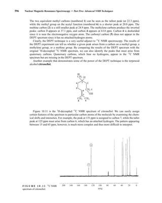
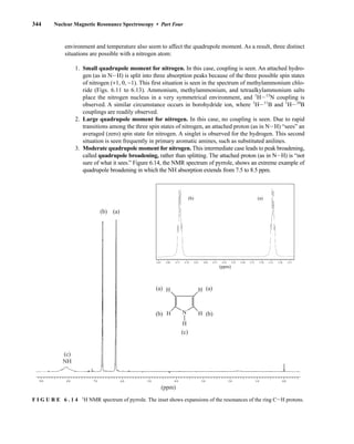
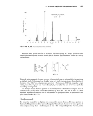
![8.8 Structural Analysis and Fragmentation Patterns 455
F I G U R E 8 . 2 9 EI mass spectrum of methylcyclopentane.
F I G U R E 8 . 3 0 EI mass spectrum of bicyclo[2.2.1]heptane (norbornane).
The mass spectra of most alkenes show distinct molecular ion peaks. Naturally, the mass of the mo-
lecular ion should correspond to a molecular formula with an index of hydrogen deficiency equal to
at least one (see Chapter 1). Apparently, electron bombardment removes one of the electrons in the π
bond, leaving the carbon skeleton relatively undisturbed. When alkenes undergo fragmentation
processes, the resulting fragment ions have formulas corresponding to CnH2n
+
and CnH2n−1
+
. It is
sometimes difficult to locate double bonds in alkenes since they migrate readily. The similarity of the
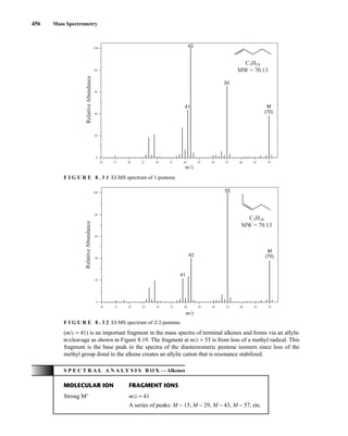
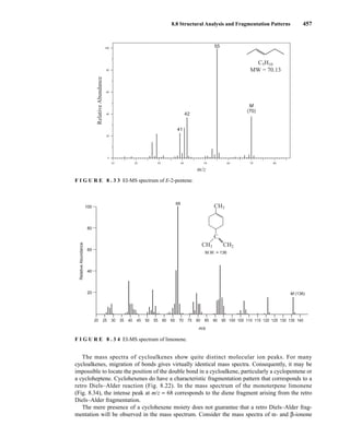
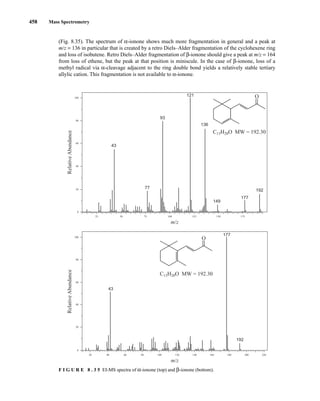
mass spectra of alkene isomers is readily seen in the mass spectra of three isomers of the formula
C5H10 (Figs. 8.31, 8.32, and 8.33). The mass spectra are very nearly identical, with the only differ-
ence being a large fragment at m/z = 42 in the spectrum of 1-pentene. This ion likely forms via loss
of ethylene through a McLafferty-type rearrangement of the molecular ion. The allyl carbocation
K. Alkenes
14782_08_Ch8_p418-519.pp3.qxd 2/6/08 3:07 PM Page 455](https://image.slidesharecdn.com/introductiontospectroscopy4ebypavia-240123161815-89f06477/85/Introduction-to-Spectroscopy-4e-by-Pavia-pdf-472-320.jpg)
![488 Mass Spectrometry
This mode of cleavage is most important for substituents attached to the number 2 position of
the ring.
•
+
•
+
N
R
CH2
N
H
CH2
CH2
H H
C
R
CH2
CH
+
m/z = 93
As is true of amines, nitrogen-bearing compounds such as amides, nitriles, and nitro compounds
must follow the Nitrogen Rule (explained more completely in Section 8.6): If they contain an odd
number of nitrogen atoms, they must have an odd-numbered molecular weight.
Amides
The mass spectra of amides usually show observable molecular ion peaks. The fragmentation pat-
terns of amides are quite similar to those of the corresponding esters and acids. The presence of a
strong fragment ion peak at m/z = 44 is usually indicative of a primary amide. This peak arises
from α-cleavage of the following sort.
Once the carbon chain in the acyl moiety of an amide becomes long enough to permit the
transfer of a hydrogen attached to the γ position, McLafferty rearrangements become possible.
For primary amides, the McLafferty rearrangement gives rise to a fragment ion peak at m/z = 59.
For N-alkylamides, analogous peaks at m/z values of 73, 87, 101, and so on often appear.
Nitriles
Aliphatic nitriles usually undergo fragmentation so readily that the molecular ion peak is too weak to
be observed. However, most nitriles form a peak due to the loss of one hydrogen atom, producing an
ion of the type RICHJ CJN+
. Although this peak may be weak, it is a useful diagnostic peak in
characterizing nitriles. In the mass spectrum of hexanenitrile (Fig. 8.76), this peak appears at m/z = 96.
•
+
•
+
H2N
H2N
H
C
O
CH2
CH2
CH2
CH2
H R
C
O CH
R
H
C
+
m/z = 59
C NH2 C NH2]
R R
O
[O
+
•
•
+
+
m/z = 44
U. Selected Nitrogen and Sulfur Compounds
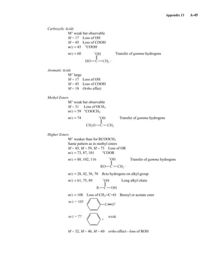
14782_08_Ch8_p418-519.pp3.qxd 2/6/08 3:08 PM Page 488](https://image.slidesharecdn.com/introductiontospectroscopy4ebypavia-240123161815-89f06477/85/Introduction-to-Spectroscopy-4e-by-Pavia-pdf-505-320.jpg)
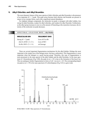
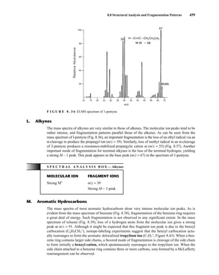
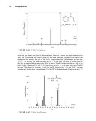
![8.8 Structural Analysis and Fragmentation Patterns 493
F I G U R E 8 . 8 1 Mass spectrum of 2-chloroheptane.
Alkyl halides may also lose a molecule of hydrogen halide according to the process
This mode of fragmentation is most important for alkyl fluorides and chlorides and is less important
for alkyl bromides and iodides. In the mass spectrum of 1-bromohexane, the peak corresponding
to the loss of hydrogen bromide at m/z = 84 is very weak. However, for 2-chloroheptane, the peak
corresponding to the loss of hydrogen chloride at m/z = 98 is quite intense.
A less important mode of fragmentation is α-cleavage, for which a fragmentation mechanism
might be
When the α position is branched, the heaviest alkyl group attached to the α carbon is lost with
greatest facility. The peaks arising from α-cleavage are usually rather weak.
A fourth fragmentation mechanism involves rearrangement and loss of an alkyl radical:
The corresponding cyclic ion can be observed at m/z = 135 and 137 in the mass spectrum of
1-bromohexane and at m/z = 105 and 107 in the mass spectrum of 2-chloroheptane. Such fragmentation
is important only in the mass spectra of long-chain alkyl chlorides and bromides.
The molecular ion peaks in the mass spectra of benzyl halides are usually of sufficient intensity to
be observed. The most important fragmentation involves loss of halogen to form the C7H7
+
ion. When
the aromatic ring of a benzyl halide carries substituents, a substituted phenyl cation may also appear.
The molecular ion peak of an aromatic halide is usually quite intense. The most important mode
of fragmentation involves loss of halogen to form the C6H5
+
ion.
CH2
CH2
CH2
CH2
R
•
•
+
+
X
CH2
CH2
CH2
CH2 R
X
+
CH2 CH2
R X R X
+
•
•
+
+
CH2 CH2
[R CH CH2]
[R
X] +
•
+
•
+
HX
14782_08_Ch8_p418-519.pp3.qxd 2/6/08 3:08 PM Page 493](https://image.slidesharecdn.com/introductiontospectroscopy4ebypavia-240123161815-89f06477/85/Introduction-to-Spectroscopy-4e-by-Pavia-pdf-510-320.jpg)