SlideShare a Scribd company logo
1 of 112
Download to read offline
Alexander Franklin Mayer
amayer@alum.mit.edu
SensibleUniverse.net
Interpreting SDSS
extragalactic data
in the era of JWST
A Full-HD Digital Monograph
James Webb Space Telescope (2022 – )
Sloan Foundation
2.5 m Telescope
Sloan Digital Sky Survey (1998 – )
© 2023–2024 A. F. Mayer
Study each page with care and attention to detail.
📄 Table of Contents
2
Review of the canonical cosmological model ..………………………………………………………………………………… 3
JWST observations………………………………………………………………………………………………………………… 7
Predictive models confronted by empirical data (6-page preview) .……………………………………………………… 12
MAGIC23 conference abstract @cern.ch.……………………………………………………………………………………… 18
Two predictive cosmological models…………………………………………………………………………………………… 19
The Sloan Digital Sky Survey (SDSS)…………………………………………………………………………………………… 24
SDSS theta-z data………………………………………………………………………………………………………………… 27
The new cosmological model….………………………………………………………………………………………………… 72
Space-density of active galactic nuclei (NED AGN) ..………………………………………………………………………… 76
SDSS, 2dF, and NED AGN data suggest fractal cosmic architecture.……………………………………………………… 85
2dF Galaxy Redshift Survey blueshifts.………………………………………………………………………………………… 92
SDSS Petrosian magnitudes (redshift-magnitude data) ……………………………………………………………………… 93
Summary .………………………………………………………………………………………………………………………… 101
‘Dark matter’……………………………………………………………………………………………………………………… 107
Quotes .…………………………………………………………………………………………………………………………… 108
The Astrophysical Journal (ApJ)..……………………………………………………………………………………………… 111
Reproducibility…………………………………………………………………………………………………………………… 112
This is a dynamic document;
click here for version check. page #
v 2024-04-09-00z
amayer@alum.mit.edu • SensibleUniverse.net
This blue is reserved for clickable 🔗.
Magenta is reserved for annotations.
A links icon on any graphic
denotes an associated link.
This document has 200+ Internet links.
Links are retrieved
using 4ref.de 🐶
🔗
Study each page with care and attention to detail.
64
• The most fundamental assumption of the Big Bang theory is that the observed
cosmological redshift of galaxies is caused by the uniform expansion of space.
• Such an expansion would cause the space between galaxies to increase over time,
which corresponds to a modeled general recessional velocity between galaxies.
• The wavelength of a receding light source is broadened towards the red end of the
visible spectrum in proportion to recession velocity, and similarly by the modeled
uniform expansion of space during light propagation; redshift is a dimensionless
quantity designated by z that is applicable to photons of any source wavelength.
• In a uniformly-expanding medium, each unit of distance expands at the same rate,
thus the recessional velocity between points is directly proportional to distance;
doubling the distance between points corresponds to doubling their relative velocity.
• Light travels at a
fi
nite speed; galaxies observed at greater distance (higher z) are
observed at greater lookback time, or farther back on the modeled cosmic timeline
from the current ‘age of the Universe’ back to the origin of that timeline at T = 0.
• If we reverse the modeled expansion, then all of the galaxies occupy a volume of
space that becomes smaller and smaller over time, culminating in a hot and dense
‘singularity’ of space and time that Sir Fred Hoyle
fl
ippantly dubbed the “Big Bang”.
3
⎧
⎪
⎨
⎪
⎩
details
next 3
pages
ca•non•i•cal (adjective) : according to recognized rules or scienti
fi
c laws [historically, often found in need of correction].
Gyr : 1 billion (109) years Gly : 1 billion (109) light years or ~1022 km …
amayer@alum.mit.edu • SensibleUniverse.net
© 2023 A. F. Mayer
The canonical uniform cosmic expansion — fundamentals
The canonical uniform cosmic expansion (A)
4
Source of the canonical numerical values: Ned Wright’s Javascript Cosmology Calculator
•L and N are equidistant from M,
and the distance L–N is 2d.
•L and M mutually recede at speed v.
•N and M mutually recede at speed v.
•L and N mutually recede at speed 2v.
d
↔︎
v , 2d
↔︎
2v , 3d
↔︎
3v … nd
↔︎
nv
v = H0·d v
2d
M
L N
d = a
∙
DC d
Big Bang
light travel time (Gyr)
comoving distance (Gly)
Observer—Now
13.2
30.7
12.8
27.5
10.4
17.2
12.2
23.9
7.8
10.9
5.8
7.3
2.5
2.7
4.3
5.1
1.3
1.4
13.7
46.4
0
0
0
∞
scale factor (1 + z)–1
0.50
1
0.33
2
0.20
4
0.14
6
0.91
0.1
0.83
0.2
0.71
0.4
0.63
0.6
1
0
a
z
t
DC
13.3
32.8
0.08
12
0.10
9
The scale factor (a) is the cosmic radius (i.e., the ‘size of the Universe’) relative to ‘now’ (1). The light travel
time (t) is the di
ff
erence between the cosmic age ‘now’ and age at z. The comoving distance DC (z) to a
particular object has a
fi
xed value over time, similar to the angle between two points on the surface of
an inflating ball. The proper distance in a particular epoch is d = a
∙
DC , so d and DC are equivalent ‘now’,
and the proper distance between galaxies at z > 12 was considerably less than 1/10th of current values.
The Hubble constant (H0) is the current-epoch (a = 1) rate of expansion, typically measured in km/s/Mpc.
© 2023 A. F. Mayer
amayer@alum.mit.edu • SensibleUniverse.net
H0 = 69.6 km·s–1·Mpc–1 ≈ 0.07c·Gly–1
ΩM = 0.286
ΩΛ = 0.714
redshift (z)
⎧
⎨
⎩ 2v
⎧
⎨
⎩
The canonical uniform cosmic expansion (B)
5
© 2023 A. F. Mayer
amayer@alum.mit.edu • SensibleUniverse.net
BB!
1. JWST observes a GALAXY at z = 9;
it has
fi
xed coordinate DC ≈ 30.7 Gly.
2. We observe that GALAXY as it
existed t ≈ 13.2 Gyr years ago
(i.e., in our distant past).
3. At that time, the age of the Universe
(i.e., the time since the Big Bang)
was about 550 Myr (T ≈ 0.55 Gyr).
4. At that time, the Universe was
1/10th (a = 0.1) the current size.
5. At that time, its distance from the
Milky Way was d = a·DC ≈ 3.1 Gly.
6. Due to cosmic expansion, its light
‘chased’ the receding Milky Way…
7. and it took t ≈ 13.2 Gyr for that light
to arrive at the JWST telescope.
8. At the current age of the cosmos
(T ≈ 13.7 Gyr), that GALAXY is now at
a distance of d = a·DC ≈ 30.7 Gly and
receding at superluminal velocity (v > c). JWST
~30.7
z = 9
GALAXY
now
z = 0
z = 0.3
z = 1
9
a = 1
a = 0.5
0.1
a ≈ 0.77
d
=
a
·
D
C
≈
3
0
.
7
Milky Way
DC ≈ 10.9
DC ≈ 3.9
DC = 0
~0.55
T ≈ 5.9
T ≈ 10.3
T ≈ 13.7
d
=
a
·
3
0
.
7
≈
2
3
.
6
d
≈
1
5
.
4
~
3
.
1
t = 0
t ≈ 3.4
t ≈ 7.8
~13.2
Milky Way
🕰
z : redshift
a : scale factor
DC : comoving distance (Gly)
d : proper distance (Gly)
T : cosmic age (Gyr)
t : light travel time (Gyr)
“lookback”
In
fl
ationary epoch
10−36 ≲ T ≲ 10−32 sec
Δa ~ 1026
Source of the canonical numerical values:
Ned Wright’s Javascript Cosmology Calculator
BB!
VIEW ANIMATION
13.2 Gly
(Gyr · c) H0 = 69.6 km·s–1·Mpc–1 ≈ 0.07c·Gly–1
ΩM = 0.286
ΩΛ = 0.714
BB!
The canonical cosmic timeline
• From 2014–2022, the “1% Concordance” model (H0 = 69.6 ± 0.7, ΩM = 0.286, ΩΛ = 0.714)
gave the much-publicized, and ostensibly well-established ‘age of the Universe’ to be
about 13.7 billion years, the value that most people today were either taught in school,
read about in a magazine, or saw in a television program or Internet science video.
• According to the latest (2022) reported “precise measurement” of the Hubble constant
(H0 = 73.30 ± 1.04) and “a consensus ΛCDM with ΩM = 0.3 and ΩΛ = 0.7”, the modeled
age of the Universe
✴︎
since the singularity has been revised, being reduced to ~12.9 Gyr.
• The ΛCDM model with the foregoing parameters correlates the measured redshift of a
galaxy (z) with the modeled age of the Universe in billions of years (T) at that redshift:
6
Big Bang
Canonical age of the Universe (Gyr) ▪︎ [1% Concordance model]
0.94
0.87
3.32
3.08
1.56
1.45
5.90
5.49
7.94
7.40
11.27
10.53
9.40
8.77
12.41
11.61
13.72
12.86
0
∞
0.50
1
0.33
2
0.20
4
0.14
6
0.91
0.1
0.83
0.2
0.71
0.4
0.63
0.6
1
0
a
z
0
0
T
0.37
0.35
0.08
12
JWST is observing
galaxies at z > 12…
0.55
0.51
0.10
9
H0 = 69.6
ΩM = 0.286
ΩΛ = 0.714
H0 = 73.30
ΩM = 0.3
ΩΛ = 0.7
JWST
© 2023 A. F. Mayer
amayer@alum.mit.edu • SensibleUniverse.net
Now
Source of the canonical numerical values: Ned Wright’s Javascript Cosmology Calculator
redshift (z)
scale factor (1 + z)–1
✴ But NOW, a new published claim [MNRAS (7 July 2023)] is 27.7 Gyr! 🤨
7
Blue Dot — Section Mark &
Return to Table of Contents
•
Companion paper: .
“Surveys with James Webb Space Telescope (JWST) have discovered candidate
galaxies in the first 400 Myr of cosmic time. … Here we identify four galaxies
located in the JWST Advanced Deep Extragalactic Survey Near-Infrared Camera
imaging with photometric redshifts z of roughly 10–13. These galaxies include the
first redshift z > 12 systems discovered with distances spectroscopically confirmed
by JWST in a companion paper.”
B. E. Robertson, S. Tacchella, B. D. Johnson, K. Hainline, L. Whitler et al.,
“Identi
fi
cation and properties of intense star-forming galaxies at redshifts
z > 10”, Nat Astron (4 April 2023).
Emma Curtis-Lake et al., Nat Astron (4 April 2023)
8
Fulvio Melina, “The Cosmic Timeline Implied by the JWST High-redshift Galaxies”,
arXiv:2302.10103 [astro-ph.CO] (20 Feb 2023).
“The so-called ‘impossibly early galaxy’ problem, first identified via the Hubble
Space Telescope’s observation of galaxies at redshifts z > 10, appears to have been
exacerbated by the more recent James Webb Space Telescope (JWST) discovery of
galaxy candidates at even higher redshifts (z ~ 17) which, however, are yet to be
confirmed spectroscopically. These candidates would have emerged only ~ 230
million years after the big bang in the context of ΛCDM, requiring a more rapid
star formation in the earliest galaxies than appears to be permitted by simulations
adopting the concordance model parameters. This time-compression problem
would therefore be inconsistent with the age-redshift relation predicted by ΛCDM.”
9
FULL ONLINE ARTICLE
10
“Deep space observations of the JWST have revealed that the structure and masses of very
early Universe galaxies at high redshifts (z ∼ 15), existing at ∼0.3 Gyr after the Big Bang,
may be as evolved as the galaxies in existence for ∼ 10 Gyr. The JWST findings are thus
in strong tension with the ΛCDM cosmological model. While tired light (TL) models
have been shown to comply with the JWST angular galaxy size data, they cannot
satisfactorily explain isotropy of the cosmic microwave background (CMB) observations
or fit the supernovae distance modulus versus redshift data well. We have developed
hybrid models that include the tired light concept in the expanding universe. The hybrid
ΛCDM model fits the supernovae type 1a data well but not the JWST observations. …”
Ivo Labbé, Pieter van Dokkum, Erica Nelson, Rachel Bezanson, Katherine A. Suess et al.,
“A population of red candidate massive galaxies ~600 Myr after the Big Bang”,
Nature (22 Feb 2023); https://doi.org/10.1038/s41586-023-05786-2.
Also see:
Michael Boylan-Kolchin, Nat Astron (13 April 2023).
Rajendra P Gupta, “JWST early Universe observations and ΛCDM cosmology”,
MNRAS (7 Jul 2023); https://doi.org/10.1093/mnras/stad2032.
1-min video
James Webb Space Telescope (JWST)
Something is amiss; the distant Universe
(z ~ 10) apparently contains big, mature
galaxies, where only “baby” galaxies are
predicted to exist so soon after T = 0.
JWST observations clearly put the ΛCDM
standard model of Big Bang cosmology
in jeopardy; has the model indeed failed?
Image credit: NASA (Artist Impression)
11
First data release
12 July 2022
Throughout this monograph:
Focal points appear in magenta.
Internet links appear in light blue.
Follow the data
& no winking…
amayer@alum.mit.edu • SensibleUniverse.net
webb.nasa.gov
‘While Hubble currently has the ability to peer billions of years into the
past to see “toddler” galaxies, the JWST will have the capability to
study “baby” galaxies, the
fi
rst galaxies that formed in the Universe.’
– esa potw1819a (7 May 2018)
😉
(references the controversial 2 Sept. 2023 NYT article)
Each model† is based on a distinct, known
exact solution of the Einstein field equations.
Model A: Einstein (1917) → ΛCDM model
Model B: de Sitter (1917) → ‘RTG’* model
Gμν + Λgμν = κTμν
12
amayer@alum.mit.edu • SensibleUniverse.net
We will compare the predictive accuracy
of two competing cosmological models.
General Audience: Ignore the unintelligible equations—they don’t matter to you;
they are like a foreign language (外語), and it is perfectly OK that you don’t know it.
* Relativistic Temporal Geometry, motivated by Minkowski (1909).
Pages 13 – 17 preview that comparison.
† The three new ‘RTG’ predictive formulas are a logically consistent set
(i.e., any one formula can be true if and only if all three formulas are true).
•
🔗
🔗 🔗
🔗
0:005 0:01 0:02 0:03 0:04 0:05 0:1 0:2 0:3 0:4 0:5 1
SpecPhoto:z (redshift)
0:2
0:3
0:4
0:5
1
2
3
4
5
10
20
30
Galaxy:
petroR50
gri
(half-light
radius
3-band
average
in
arcsec)
ΛCDM
predictive curves
13
0.32
0.08
0.02
amayer@alum.mit.edu • SensibleUniverse.net • Data: SDSS
smallest
galaxies
10×
reference
petroR50_gri
--- ΛCDM curves
H0 = 69.6
ΩM = 0.286
ΩΛ = 0.714
“theta = size / DA”
--- θ
̅z data
As per di
ff
erences in ‘measurements’ of (H0, ΩM, ΩΛ), such variation has no appreciable e
ff
ect on these curves.
intercept
62←
⎧
⎪
⎨
⎪
⎩
Wright (2006)
~2.4M measurements
Empirical reference curve
(constant intrinsic-galaxy-size
as per linear
fi
t to data points)
The data does not support the model;
the ΛCDM model fails catastrophically.*
*This model is
irreconcilable
with the data.
z-bin
Apparent size vs. redshift
0:005 0:01 0:02 0:03 0:04 0:05 0:1 0:2 0:3 0:4 0:5 1
SpecPhoto:z (redshift)
0:2
0:3
0:4
0:5
1
2
3
4
5
10
20
30
Galaxy:
petroR50
gri
(half-light
radius
3-band
average
in
arcsec)
petroR50_gri
14
θ(z) = Cℓ
(
1 −
1
(z + 1)2 )
−1
2
, Cℓ = 1
0.32
0.08
0.02 0.64
0.16
0.04
0.01
--- θ(z)
--- θ
̅z data
amayer@alum.mit.edu • SensibleUniverse.net • Data: SDSS
There are no free parameters to modify the curve;
Cℓ merely shifts the curve up or down on the θ-axis.
(remarkably, not an arbitrary #)
The RTG predictive model
fi
ts the data.
Cℓ = 2
Cℓ = 0.5
1
reference
constants
69←
N = 398 3.5k 8.3k 38.8k 34.7k 36.5k 7.1k
Bin galaxies:
[constant intrinsic galaxy size]
Minimal-data
measurement
z-bin
Apparent size vs. redshift
VC(z)
N(z)
Cumulative
AGN
count
102
103
104
105
106
109
Comoving
volume
V
C
(
VSmoots
)
103
106
109
Redshift (z)
0.01 0.1 1 10
The third and quite certain interpretation
of the graph is that this redshift-volume
model [VC(z)] is radically unphysical.
3︎⃣
ρAGN
7.40E–5
ΛCDM: over time, AGN space density increases by ~4 orders of magnitude.
Another possible interpretation of the graph, is that ≪1% of AGN that exist at
higher redshift are observed and counted by the various astronomical surveys.
15
ρAGN
1
ρAGN =
N(z)
VC(z)
ΛCDM Lookback: 140 Myr ΛCDM Lookback: 12.86 Gyr
6.42
H0 = 69.6
ΩM = 0.286
ΩΛ = 0.714
1︎⃣2︎⃣
Δzbin = 0.001
[arbitrary
units]
The data does not support the model;
the ΛCDM model fails catastrophically.
amayer@alum.mit.edu • SensibleUniverse.net • Data: NED
81←
(for
intercept)
>4
orders
of
magnitude!
Volume/AGN vs. redshift
ΛCDM: cosmic galaxy evolution over ~12.7 Gyr
S3
(z)
N(z)
Cumulative
AGN
count
102
103
104
105
106
109
Proper
volume
(arbitrary
units)
103
106
109
Redshift (z)
0.01 0.1 1 10
S3
(z) = CV ⋅ cos−1
(
1
z + 1)
−
(
1
(z + 1)2
−
1
(z + 1)4 )
1
2
S3 represents the volumetric ‘surface’ of a Riemannian 3-sphere
The
fi
t of this a priori theoretical predictive curve to the empirical AGN population data is equally
remarkable to that for the theta-z data; there are no free parameters available to achieve this
fi
t.
16
Δzbin = 0.001
same
intercept
amayer@alum.mit.edu • SensibleUniverse.net • Data: NED
82←
CV
= 9.7E4
(sets the intercept)
Volume/AGN vs. redshift
The RTG predictive model
fi
ts the data.
The interpretation of this graph is that AGN are accurately
counted, even out to very high redshift, and that galaxy clusters
comprise a
fi
xed percentage of AGN throughout the Universe.
intercepts
(0.32, 18.2)
(0.32, 16.6)
Redshift-magnitude curves modeling constant intrinsic brightness
17
Note: g-band data must exhibit 4000 Å break!
Data: ~136k
SDSS LRGs (z-band)
RTG: m(z) = CM − 2.5 log
[
1
4π ((z + 1)4 − (z + 1)2
) ]
+ ϵλ ⋅ cos−1
(
1
z + 1)
−
CM = 14.82, 13.22 ϵλ = 0.5 CM = 15.17, 13.57 ϵλ = 0
−
−
ΛCDM: m(z) = KM − 2.5 log
[
1
4πD2
L ]
−
KM = − 0.68, − 2.28
amayer@alum.mit.edu • SensibleUniverse.net • Data: SDSS
97←
The SDSS Luminous Red Galaxies (LRGs)
were speci
fi
cally selected to have similar
characteristics, including their luminosity.
extinction
RTG constant-intrinsic-brightness model
The RTG predictive model
fi
ts the data.
ΛCDM
constant-intrinsic-brightness model
The data does not support this model.*
* The ΛCDM model fails catastrophically.
https://indico.cern.ch/event/1153372/contributions/5200955/
18
“Facts do not cease to exist because they are ignored.”
– Aldous Huxley (1927)
•
of
~
🔗
End of preview; Main Presentation • ⤺Table of Contents
What is Science?
(2-minute video)
– Yuri Ivanovich Manin, Talk on Computability, Northwestern University (c. 1995)
“When I was starting out in mathematics, it seemed very important
to prove a big theorem. Now, with more experience, I understand
that it is new notions that are more important, for example, Alan
Turing’s new notion of computability, which I shall discuss today.”
19
amayer@alum.mit.edu • SensibleUniverse.net
I thank Dr. Michael Stephen Fiske, Ph.D. Mathematics, Northwestern (1996) for this quotation.
•
As per this quote that Dr. Fiske had previously shared with me, I contacted Yuri, and he
then invited me to meet with him at his o
ffi
ce at the Max-Planck-Institut für Mathematik in
Bonn on 14 August 2009. We spoke about mathematical physics in a cordial discussion
of well over two hours in which I
fi
lled three whiteboards with equations and diagrams.
Our discussion concluded with Yuri memorably re
fl
ecting on the fact that his contributions
to
fi
eld theory represented a signi
fi
cant lifetime investment — read between the lines.
Best Paper Award
HICSS 2022 & 2023
ψ
ψ
20
Spherical coordinate system (r, θ, ψ)
amayer@alum.mit.edu • SensibleUniverse.net
The following page (21) presents Einstein’s 1917 exact
solution of the
fi
eld equations in the form of a metric
(i.e., an equation that measures distance).
It is important to understand that the locally-de
fi
ned
blue vector r here is the same dimension of physical
space as the blue arc r on page 21, and that the dot at
the origin here can represent any point on the circle.
The interior region of the blue circle of radius R does
not represent space; the other two space dimensions
(θ, ψ), over which distances between galaxies can be
measured, are not represented in the diagram.
We call the Euclidean coordinate system on the left,
which represents strictly-locally-de
fi
ned measurable
3-dimensional physical space, a tangent space.
Each such tangent space has a 4th coordinate, t that
represents time as locally measured in that space; t is
mutually orthogonal to the three space coordinates in
accord with the locally-applicable Minkowski metric.
ds2
= x2
+ y2
+ z2
+ (ict)2
local Minkowski metric
Note that i2 = –1
This Euclidean coordinate system
is valid only in the neighbourhood
of its own origin at r = 0.
page-21 preview
r
R
s
p
a
ce
Milky Way
Distant
Galaxy
Model (“System”) A
Einstein’s metric —an exact solution of the Einstein
fi
eld equations (EFE)
21
t
r
R
Riemannian geometry
vs.
Euclidean geometry
amayer@alum.mit.edu • SensibleUniverse.net
✓
R ∝ a (dimensionless cosmic scale factor)
The blue circle represents a cosmological great circle — a single
dimension of measurable physical space in two dimensions of ℝ4.
ℝ4 means a 4D Euclidean
space, which may contain
a 4-dimensional sphere.
ds2
= − dr2
− R2
sin2
(
r
R) [dψ2
+ sin2
(ψ) dθ2
] + c2
dt2
dθ = dΨ = 0
χ ≡
r
R
χ ∝ DC
χ
© 2023 A. F. Mayer
A. Einstein, “Cosmological Considerations in the General Theory of Relativity”, SPAW, 142 (1917).
✓
1) The Universe is
fi
nite, yet has no boundary.
2) Time is independent of space in the metric.
equivalence
proportionality
58←
& symmetry!
s
p
a
ce
1-minute
VIDEO
Milky Way
Distant
Galaxy
– Willem de Sitter (31 March 1917)
“We thus find that in the System A the time has a separate position.
That this must be so, is evident a priori. For speaking of the three-
dimensional world, if not equivalent to introducing an absolute time, at
least implies the hypothesis that at each point of the four-dimensional
space there is one absolute coordinate x4 which is preferable to all
others to be used as “time”, and that at all points and always this one
coordinate is actually chosen as time. Such a fundamental difference
between the time and the space-coordinates seems to be somewhat
contradictory to the complete symmetry of the field-equations…”
W. de Sitter, “On the relativity of inertia. Remarks concerning Einstein’s latest hypothesis”,
KNAW Proceedings 19(2), 1217 (1917).
22
amayer@alum.mit.edu • SensibleUniverse.net
Referencing Einstein’s metric, expressed using x4 ≡ t
⎫
⎪
⎬
⎪
⎭
W. de Sitter,
“Einstein’s theory of gravitation and its astronomical consequences. Third paper”, MNRAS 78, 3 (1917).
Model B
Willem de Sitter’s metric — a different exact solution of the EFE
23
This interpretation of de Sitter’s metric, where
time is a strictly-local geometric object is new.
It also elegantly resolves the quandary of zero
cosmic matter density imposed by this solution.
amayer@alum.mit.edu • SensibleUniverse.net
dρ2 = − dρ1 ∴
∫
2π
0
dρ = ρ = 0
Cosmic perspective
relativistic perspective
density
ds2
= − dr2
− R2
sin2
(
r
R) [dψ2
+ sin2
(ψ) dθ2
] + cos2
(
r
R )
c2
dt2
c2dτ2
locally
dρ1 > 0
locally
dρ2 > 0
dρn is local
mass-energy
density
t
τ
r
R
1
2
cos
(
r
R)
= cos χ =
dτ
dt
energetic
relationship
→
1) The Universe is
fi
nite, yet has no boundary.
2) Time is dependent on space in the metric.
© 2023 A. F. Mayer 65←
·
R = 0
χ
dθ = dΨ = 0
χ ≡
r
R
“In 1987 Gunn proposed putting an array
of CCDs on a 2.5m-telescope…”
J. E. GUNN ET AL.,
“The 2.5 m Telescope of the Sloan Digital Sky Survey”,
The Astronomical Journal, 131:2332–2359, 2006 April.
24
Creative Innovator & Leader
PRINCETON UNIVERSITY
Adapted from a screen shot of Gunn’s o
ffi
cial web page at Princeton.
•
photo credit: Reidar Hahn, Fermilab Visual Media Services
Sloan Foundation
2.5-m Telescope
Sloan Digital Sky Survey
SDSS.org
25
Apache Point Observatory
Sunspot, New Mexico, USA
26
“The core of science is not mathematical modeling; it is intellectual honesty. It is a
willingness to have our certainties about the world constrained by good evidence
and good argument.”
⋮
“Either a person is being intellectually honest, or he isn’t. Either a person is willing
to look dispassionately at the data or he is trying to conform the data to his prior
conception of the world. And science, when it is working, which is to say when it
is really science, amounts to a systematic eschewal of dogma. I mean, dogma in
science is humiliating, whenever it is recognized to be dogma.”
– Sam Harris
Beyond Belief: Science, Reason, Religion & Survival, Salk Institute (Nov 2006)
Also appearing at the conference, Neil deGrasse Tyson
amayer@alum.mit.edu • SensibleUniverse.net
🌱 ⚰
Theories live and die by accurate empirical data.
27
•
ac·cu·rate (adjective) : faithfully or fairly representing the truth about someone or something.
“Scientists are more readily bought than politicians.” – anon.
annotation
28
edwardtufte.com
0:005 0:01 0:02 0:03 0:04 0:05 0:1 0:2 0:3 0:4 0:5 1
SpecPhoto:z (redshift)
0:2
0:3
0:4
0:5
1
2
3
4
5
10
20
30
Galaxy:
petroR50
gri
(half-light
radius
3-band
average
in
arcsec)
BLUE DOT REPRESENTS ONE GALAXY
BLUE: sparser data → RED: denser data
Theta-z log-log plot of half-light radius (petroR50) for ~800k galaxies
Measured
apparent
radius
(arcsec)
29
Low-z
⬅︎
NEARER
High-z
FARTHER
➡︎
SMALLER
⇩
⇧
LARGER
z = 0.32
z = 0.08
z = 0.02 z = 1
z = 0.01
Theta-z ≡ “apparent size versus redshift”
amayer@alum.mit.edu • SensibleUniverse.net • Data: SDSS
Color scaling is log2.
Blue dot 1 galaxy
Cyan dot 2 galaxies
Yellow dot 4 galaxies
Red dot 8 galaxies
Source: Glossary of SDSS-IV Terminology
SDSS glossary reference
petroRad
The Petrosian radius. A measure of the angular size of an
image, most meaningful for galaxies. Units are seconds of arc.
The Petrosian radius (and related measures of size called
petroR50 and petroR90) are derived from the surface
brightness profile of the galaxy, as described in Algorithms.
Surface Brightness
The frames pipeline also reports the radii containing 50% and
90% of the Petrosian flux for each band, petroR50 and
petroR90 respectively. …
30
Understanding SDSS angular resolution (“theta” measurement)
Average apparent diameter of full Moon at zenith: 31.6′ = 1896ʺ.
Compared relative to the average apparent size of the full Moon, the green dot
has a 10ʺ diameter; that same size is also compared to a z ~ 0.08 SDSS galaxy.
31
© 2016–2023 A. F. Mayer
Click image for SDSS SkyServer Explorer.
10ʺ
ObjID: 1237658298990330048
petroRad_gri = 18.5±0.3ʺ
Petrosian radius
∴
petroRad
circle encloses
~7k CCD pixels
–
petroR50
circle encloses
~2k CCD pixels
rP
petroR50_gri = 9.8±0.1ʺ
half-light radius z = 0.0762
0.396 arcsec∙pix–1
OPTICAL NEGATIVE
amayer@alum.mit.edu • SensibleUniverse.net
🌎
Apogee
(29.9′
)
Perigee
(33.5′
)
Semimajor
axis
(31.6′
)
Earth-Moon System to scale
green dot
🔗
Reference:
r
The observed radial galaxy brightness pro
fi
le [ I(r′) ] is
“azimuthally averaged” (i.e., averaged over 2π radians).
≡
d ′
r 2π ′
r I ′
r
( )/ π 1.252
− 0.82
( )r2
0.8r
1.25r
∫
d ′
r 2π ′
r I ′
r
( )/ πr2
0
r
∫
𝓡
P(r)
local surface brightness
in annulus (blue region)
0.8r r 1.25r
Here, r is a variable measurement;
it is not a recorded measurement.
DEFINITION: “Petrosian ratio” [
𝓡
P(r)]
1.25r
0.8r
mean surface brightness
measured inside radius r
÷
Define
𝓡
P,lim as
𝓡
P(rP) =
𝓡
P,lim where rP is the
measured and recorded Petrosian radius.
𝓡
P,lim = 0.2 for the SDSS:
Varying r, when
𝓡
P(r) = 0.2, then rP = r.
Petrosian radius (SDSS “petroRad” measurement)
32
© 2015–2023 A. F. Mayer
amayer@alum.mit.edu • SensibleUniverse.net
𝓡
P(r) ≡
Measures Of Flux And Magnitude – Petrosian Magnitudes: petroMag
0:005 0:01 0:02 0:03 0:04 0:05 0:1 0:2 0:3 0:4 0:5 1
SpecPhoto:z (redshift)
0:2
0:3
0:4
0:5
1
2
3
4
5
10
20
30
Galaxy:
petroR50
gri
(half-light
radius
3-band
average
in
arcsec)
ObjID: 1237658298990330048
33
SDSS 18
finding chart
Every galaxy plotted includes this basic empirical data and far more.
Click for more data…
theta-z coordinates of this galaxy (petroR50_gri)
OPTICAL NEGATIVE
amayer@alum.mit.edu • SensibleUniverse.net • Data: SDSS
SDSS SkyServer Database Values (arcsec)
petroRad_g 18.22892±0.27
petroRad_r 18.69740±0.31
petroRad_i 18.64179±0.35
petroRad_gri 18.52±0.31
petroR50_g 9.70912±0.11
petroR50_r 9.77527±0.06
petroR50_i 9.83906±0.05
petroR50_gri 9.77±0.08
z 0.076242
zErr 2.46E-05
🔗
Ultraviolet
u
Green
g
Red
r
Near Infrared
i
Infrared
z
3531 4627 6140 7467 8887
Central wavelengths λeff (Å) from Doi et al. (2010),Table 2.
SDSS astronomical band-pass
fi
lters λeff (Å)
Not redshift (z)!
photo credit: Michael Carr
photo credit: Smithsonian National Air and Space Museum
34
disambiguation for a general audience
Click for article…
amayer@alum.mit.edu • SensibleUniverse.net
🔗
0:005 0:01 0:02 0:03 0:04 0:05 0:1 0:2 0:3 0:4 0:5 1
SpecPhoto:z (redshift)
0:2
0:3
0:4
0:5
1
2
3
4
5
10
20
30
Galaxy:
petroR50
gri
(half-light
radius
3-band
average
in
arcsec)
~2.4×10⁶ Empirical Measurements
35
~2.4 MILLION measurements
There are 795,838 galaxies (data) represented in this graph, and each
datum represents the average of 3 distinct (g, r, i) radius measurements.
Too many measurements to “massage”
the data according to con
fi
rmation bias.
0.32 1
0.08
0.02
0.01
amayer@alum.mit.edu • SensibleUniverse.net • Data: SDSS
Apparent size vs. redshift
0:005 0:01 0:02 0:03 0:04 0:05 0:1 0:2 0:3 0:4 0:5 1
SpecPhoto:z (redshift)
0:2
0:3
0:4
0:5
1
2
3
4
5
10
20
30
Galaxy:
petroR50
gri
(half-light
radius
3-band
average
in
arcsec) 36
smallest
galaxies
10×
reference
petroR50_gri
0.32 1
0.08
0.02
0.01
SDSS cannot see the smallest
galaxies at this great distance.
Far away, the faint outer regions of the largest
galaxies are not seen, so they appear smaller.
Galaxies at the peak of each reference rod are 10×
greater in measured radius than those at the base.
amayer@alum.mit.edu • SensibleUniverse.net • Data: SDSS
The intrinsic radial size of typical galaxies,
including all morphologies, spans an order of
magnitude (i.e., ×10), which decadal range
excludes statistically-unlikely outliers.
①
37
Empirical Inference
Inference | ˈinf(ə)rəns |
noun
a conclusion reached on the basis of evidence and reasoning: researchers are
entrusted with drawing inferences from the data.
amayer@alum.mit.edu • SensibleUniverse.net
0:005 0:01 0:02 0:03 0:04 0:05 0:1 0:2 0:3 0:4 0:5 1
SpecPhoto:z (redshift)
0:2
0:3
0:4
0:5
1
2
3
4
5
10
20
30
Galaxy:
petroR50
gri
(half-light
radius
3-band
average
in
arcsec) 38
×2 ×2 ×2 ×2 ×2 ×2
7 Redshift (z
̅) Bins
Each bin allows us to examine a group of
galaxies that are close to each other in
redshift (i.e., at about the same distance).
amayer@alum.mit.edu • SensibleUniverse.net • Data: SDSS
0.01
0.02
0.04
0.08
0.16
0.32
0.64
z
̅ =
398
3.5k
8.3k
38.8k
34.7k
36.5k
7.1k
N ≊
galaxy
count
average
redshift
0:0760 0:0765 0:0770 0:0775 0:0780 0:0785 0:0790 0:0795 0:0800 0:0805 0:0810 0:0815 0:0820 0:0825 0:0830 0:0835 0:0840
SpecPhoto:z (redshift)
1
2
3
4
5
10
Galaxy:
petroR50
gri
(half-light
radius
3-band
average
in
arcsec) 39
Measurement-error ellipses for z
̅ = 0.080 (5% regular sample of the bin)
0.760 0.084
0.080
Measured
apparent
radius
(arcsec)
Redshift (z)
nth selection sample interval = 20
amayer@alum.mit.edu • SensibleUniverse.net • Data: SDSS
0:304 0:306 0:308 0:310 0:312 0:314 0:316 0:318 0:320 0:322 0:324 0:326 0:328 0:330 0:332 0:334 0:336
SpecPhoto:z (redshift)
1
2
3
4
5
10
Galaxy:
petroR50
gri
(half-light
radius
3-band
average
in
arcsec) 40
0.304 0.336
0.320
Measurement-error ellipses for z
̅ = 0.320 (5% regular sample of the bin)
nth selection sample interval = 20
amayer@alum.mit.edu • SensibleUniverse.net • Data: SDSS
0:005 0:01 0:02 0:03 0:04 0:05 0:1 0:2 0:3 0:4 0:5 1
SpecPhoto:z (redshift)
0:2
0:3
0:4
0:5
1
2
3
4
5
10
20
%petroR50Err
gri
(radius
measurement
error
as
a
%
of
measurement)
Radius measurement error (petroR50Err) as a percent of the measurement
41
20% pop.
at z ≥ 0.310
80%
pop.
10%
5%
1%
Error
%
1
0.08
0.02
0.01 0.32
amayer@alum.mit.edu • SensibleUniverse.net • Data: SDSS
0:005 0:01 0:02 0:03 0:04 0:05 0:1 0:2 0:3 0:4 0:5 1
SpecPhoto:z (redshift)
0:2
0:3
0:4
0:5
1
2
3
4
5
10
20
30
Galaxy:
petroR50
gri
(half-light
radius
3-band
average
in
arcsec)
A Massive Volume of High-Quality Data
Principle galaxy selection criteria:
•Maximum allowed radius-measurement
error in any of the three bands is 20%.
•Maximum allowed redshift error is 1%.
Plotted theta-z data set:
•Average gri radius-measurement error is 3.6%.
•Average redshift-measurement error is 0.021%.
42
amayer@alum.mit.edu • SensibleUniverse.net
0:005 0:01 0:02 0:03 0:04 0:05 0:1 0:2 0:3 0:4 0:5 1
SpecPhoto:z (redshift)
0:2
0:3
0:4
0:5
1
2
3
4
5
10
20
30
Galaxy:
petroR50
gri
(half-light
radius
3-band
average
in
arcsec)
✓
Minimum Redshift
zmin
Maximum Redshift
zmax
Average Redshift Galaxy count
N
StdDev[ ln(r) ]
σ
ln(r)
µ
Mean Radius Median Radius Standard Deviation
0.0090 0.0110 0.010 398 0.6711 1.5170 5.71 4.56 1.96
0.0180 0.0220 0.020 3,483 0.5593 1.3984 4.73 4.05 1.75
0.0380 0.0420 0.040 8,345 0.4686 1.1179 3.41 3.06 1.60
0.0760 0.0840 0.080 38,831 0.3870 0.8200 2.45 2.27 1.47
0.1520 0.1680 0.160 34,762 0.2952 0.7156 2.14 2.05 1.34
0.3040 0.3360 0.320 36,487 0.2297 0.4503 1.61 1.57 1.26
0.6100 0.6780 0.640 7,147 0.2236 0.1637 1.21 1.18 1.25
θ = e(μ+σ2
2 )
z =
∑
z ÷ N eμ
eσ
43
log-normal distribution
Redshift Bin Statistics for petroR50_gri (Geometric vs. Arithmetic)
normal distribution✗
amayer@alum.mit.edu • SensibleUniverse.net • Data: SDSS
Bin Count (galaxies)
Median Radius (4.56)
Mean Radius (5.71)
Radius-Bin
Count
(n)
0
5
10
15
20
Galaxy.petroR50_gri (arcsec)
0.5 1 2 5 10 20
Empirical Galaxy-Size Distribution
Not much useful data
here at low-redshift…
😰
44
0:005 0:01 0:02 0:03 0:04 0:05 0:1 0:2 0:3 0:4 0:5 1
SpecPhoto:z (redshift)
0:2
0:3
0:4
0:5
1
2
3
4
5
10
20
30
Galaxy:
petroR50
gri
(half-light
radius
3-band
average
in
arcsec)
amayer@alum.mit.edu • SensibleUniverse.net
z
̅ = 0.010
N = 398 ( ∑n )
Δrbin = 0.1″
NOTE:
This redshift (0.010) is 3 times
greater than the maximum z in
Edwin Hubble’s 1929 diagram.
45
NO WORRIES,
SDSS HAS AN
EXCELLENT
TELESCOPE
AND A TEAM OF
OUTSTANDING
ASTRONOMERS…
😎
photo credit:
Reidar Hahn, Fermilab Visual Media Services
μ = 1.3984
σ = 0.5593
S = 350 (scaling constant)
Bin Count (galaxies)
Median Radius (4.05)
Mean Radius (4.73)
PDF*: fX(r; μ, σ) ⋅ S
Radius-Bin
Count
(n)
0
50
100
150
200
Galaxy.petroR50_gri (arcsec)
0.5 1 2 5 10 20
* Probability Density Function
Note: the vertical scale is
>10× the z
̅ = 0.010 scale.
46
N = 3,483 ( ∑n )
Empirical Galaxy-Size Distribution vs. Analytic Log-Normal Distribution Curve
0:005 0:01 0:02 0:03 0:04 0:05 0:1 0:2 0:3 0:4 0:5 1
SpecPhoto:z (redshift)
0:2
0:3
0:4
0:5
1
2
3
4
5
10
20
30
Galaxy:
petroR50
gri
(half-light
radius
3-band
average
in
arcsec)
z
̅ = 0.020
fX(r; μ, σ) =
1
rσ 2π
exp −
(ln r − μ)
2
2σ2
Δrbin = 0.1″
amayer@alum.mit.edu • SensibleUniverse.net • Data: SDSS
μ = 1.1179
σ = 0.4686
S = 800
Bin Count (galaxies)
Median Radius (3.06)
Mean Radius (3.41)
PDF: fX(r; μ, σ) ⋅ S
Radius-Bin
Count
(n)
0
100
200
300
400
Galaxy.petroR50_gri (arcsec)
0.5 1 2 5 10 20
Note: the vertical scale is
2× the z
̅ = 0.020 scale.
47
0:005 0:01 0:02 0:03 0:04 0:05 0:1 0:2 0:3 0:4 0:5 1
SpecPhoto:z (redshift)
0:2
0:3
0:4
0:5
1
2
3
4
5
10
20
30
Galaxy:
petroR50
gri
(half-light
radius
3-band
average
in
arcsec)
z
̅ = 0.040
N = 8,345 ( ∑n )
Empirical Galaxy-Size Distribution vs. Analytic Log-Normal Distribution Curve
Δrbin = 0.1″
amayer@alum.mit.edu • SensibleUniverse.net • Data: SDSS
μ = 0.8200
σ = 0.3870
S = 3850
Bin Count (galaxies)
Median Radius (2.27)
Mean Radius (2.45)
PDF: fX(r; μ, σ) ⋅ S
Radius-Bin
Count
(n)
0
1k
2k
3k
4k
Galaxy.petroR50_gri (arcsec)
0.5 1 2 5 10 20
Note: the vertical scale is
10× the z
̅ = 0.040 scale.
48
z
̅ = 0.080
0:005 0:01 0:02 0:03 0:04 0:05 0:1 0:2 0:3 0:4 0:5 1
SpecPhoto:z (redshift)
0:2
0:3
0:4
0:5
1
2
3
4
5
10
20
30
Galaxy:
petroR50
gri
(half-light
radius
3-band
average
in
arcsec)
N = 38,831 ( ∑n )
Empirical Galaxy-Size Distribution vs. Analytic Log-Normal Distribution Curve
Δrbin = 0.1″
amayer@alum.mit.edu • SensibleUniverse.net • Data: SDSS
μ = 0.7156
σ = 0.2952
S = 3700
Bin Count (galaxies)
Median Radius (2.05)
Mean Radius (2.14)
PDF: fX(r; μ, σ) ⋅ S
Radius-Bin
Count
(n)
0
1k
2k
3k
4k
Galaxy.petroR50_gri (arcsec)
0.5 1 2 5 10 20
49
z
̅ = 0.160
0:005 0:01 0:02 0:03 0:04 0:05 0:1 0:2 0:3 0:4 0:5 1
SpecPhoto:z (redshift)
0:2
0:3
0:4
0:5
1
2
3
4
5
10
20
30
Galaxy:
petroR50
gri
(half-light
radius
3-band
average
in
arcsec)
N = 34,762 ( ∑n )
Note: the vertical scale
now remains constant…
Empirical Galaxy-Size Distribution vs. Analytic Log-Normal Distribution Curve
Δrbin = 0.1″
amayer@alum.mit.edu • SensibleUniverse.net • Data: SDSS
μ = 0.4503
σ = 0.2297
S = 3900
Bin Count (galaxies)
Median Radius (1.57)
Mean Radius (1.61)
PDF: fX(r; μ, σ) ⋅ S
Radius-Bin
Count
(n)
0
1k
2k
3k
4k
Galaxy.petroR50_gri (arcsec)
0.5 1 2 5 10 20
50
z
̅ = 0.320
0:005 0:01 0:02 0:03 0:04 0:05 0:1 0:2 0:3 0:4 0:5 1
SpecPhoto:z (redshift)
0:2
0:3
0:4
0:5
1
2
3
4
5
10
20
30
Galaxy:
petroR50
gri
(half-light
radius
3-band
average
in
arcsec)
N = 36,487 ( ∑n )
Empirical Galaxy-Size Distribution vs. Analytic Log-Normal Distribution Curve
Δrbin = 0.1″
amayer@alum.mit.edu • SensibleUniverse.net • Data: SDSS
μ = 0.1637
σ = 0.2236
S = 700
Bin Count (galaxies)
Median Radius (1.18)
Mean Radius (1.21)
PDF: fX(r; μ, σ) ⋅ S
Radius-Bin
Count
(n)
0
1k
2k
3k
4k
Galaxy.petroR50_gri (arcsec)
0.5 1 2 5 10 20
51
z
̅ = 0.640
0:005 0:01 0:02 0:03 0:04 0:05 0:1 0:2 0:3 0:4 0:5 1
SpecPhoto:z (redshift)
0:2
0:3
0:4
0:5
1
2
3
4
5
10
20
30
Galaxy:
petroR50
gri
(half-light
radius
3-band
average
in
arcsec)
N = 7,147 ( ∑n )
Empirical Galaxy-Size Distribution vs. Analytic Log-Normal Distribution Curve
Δrbin = 0.1″
amayer@alum.mit.edu • SensibleUniverse.net • Data: SDSS
Galaxies have a log-normal size distribution.
②
52
Empirical Inference
amayer@alum.mit.edu • SensibleUniverse.net
Shiyin Shen, H. J. Mo, Simon D. M. White, Michael R. Blanton, Guinevere Kauffmann et al., “The size
distribution of galaxies in the Sloan Digital Sky Survey”, Mon. Not. R. Astron. Soc. 343, 978 (2003).
The foregoing analysis generalizes an earlier
fi
nding dating back two decades:
That distribution is empirically observed to be
consistent over the data set (0.02 ≤ z ≤ 0.64).
③
53
Empirical Inference
amayer@alum.mit.edu • SensibleUniverse.net
To very good approximation, the mean apparent
galaxy size (theta-bar) in each redshift bin can
be expected to represent the same standard rod
(i.e., to be very nearly the same intrinsic size ℓ).
④
54
Inference | ˈinf(ə)rəns |
noun
a conclusion reached on the basis of evidence and reasoning: researchers are
entrusted with drawing inferences from the data.
Empirical Inference
amayer@alum.mit.edu • SensibleUniverse.net
0:005 0:01 0:02 0:03 0:04 0:05 0:1 0:2 0:3 0:4 0:5 1
SpecPhoto:z (redshift)
0:2
0:3
0:4
0:5
1
2
3
4
5
10
20
30
Galaxy:
petroR50
gri
(half-light
radius
3-band
average
in
arcsec) 55
Galaxy Mean Radius (θ
̅z) Plotted For Each Redshift Bin (Black Squares)
0.01
0.02
0.04
0.08
0.16
0.32
0.64
z
̅ =
amayer@alum.mit.edu • SensibleUniverse.net • Data: SDSS
398
3.5k
8.3k
38.8k
34.7k
36.5k
7.1k
N ≊
Radius-bin
count(n)
0
1000
2000
3000
4000
Galaxy.petroR50_gri (arcsec)
0.6 0.8 1 2 4 6 8 10 12 16
sample galaxy image
56
z = 0.076
z = 0.084
θ
̅
=
2.45″
Δrbin = 0.2″
ObjID: 1237665101141835997 🔗
N = 38,831 galaxies (each dot is a galaxy)
bin slice →
Color denotes data density; color scaling is log2.
z
̅ = 0.08 redshift-bin
Δsize = 10
Same data as page 48, but
a montage with more detail
and di
ff
erent (×2) Δrbin.
5″ 20″
petroR50_gri 2.450 (120 pix)
petroRad_gri 5.124 (526 pix)
z 0.0794
petroR50_gri 11.54 ( 2.7k pix)
petroRad_gri 28.68 (16.5k pix)
z 0.0789
ObjID: 1237678617430589483 🔗
Measurement
exaggerated
by environs.
amayer@alum.mit.edu • SensibleUniverse.net • Data: SDSS
5 extreme outliers
⎧
⎪
⎨
⎪
⎩
Click
image
for
Skyserver…
0:005 0:01 0:02 0:03 0:04 0:05 0:1 0:2 0:3 0:4 0:5 1
SpecPhoto:z (redshift)
0:2
0:3
0:4
0:5
1
2
3
4
5
10
20
30
Galaxy:
petroR50
gri
(half-light
radius
3-band
average
in
arcsec)
Empirical Constant-Intrinsic-Galaxy-Size Curve (linear
fi
t to θ
̅z data)
log θ = − 0.3749 ⋅ log z + 0.01355
--- θ
̅z data
Empirical reference curve
(constant intrinsic-galaxy-size
as per linear
fi
t to data points)
0.32
0.08
0.02
0.01 1
0.04 0.16 0.64
3× Hubble’s
maximum z
amayer@alum.mit.edu • SensibleUniverse.net • Data: SDSS
Pearson correlation coefficient: – 0.9967
57
(–1 implies a perfect linear relationship.)
58
t
Riemannian geometry
vs.
Euclidean geometry
ds2
= − dr2
− R2
sin2
(
r
R) [dψ2
+ sin2
(ψ) dθ2
] + c2
dt2
amayer@alum.mit.edu • SensibleUniverse.net
A. Einstein, “Cosmological Considerations in the General Theory of Relativity”, SPAW, 142 (1917).
✓
Recall
(page 21)
Galaxy redshift & time dilation modeled
as dR/dt > 0 (i.e., “expanding universe”).
r
R(t)
R ∝ a (dimensionless cosmic scale factor)
Model (“System”) A
Einstein’s metric —an exact solution of the Einstein
fi
eld equations (EFE)
χ
✓
1) The Universe is
fi
nite, yet has no boundary.
2) Time is independent of space in the metric.
© 2023 A. F. Mayer
dθ = dΨ = 0
χ ≡
r
R
χ ∝ DC
& symmetry!
21→
s
p
a
ce
1-minute
VIDEO
z = 0.0033
Hubble Diagram (1929) — Annotated
E. Hubble,
“A Relation between Distance and Radial Velocity among Extra-Galactic Nebulae”, PNAS 15, 168 (1929).
Hubble constant
modern value*
H0 = 69.6 ± 0.7
*Recently updated
H0 = 73.30 ± 1.04
(q0 = –0.51 ± 0.024)
H0 = 530
amayer@alum.mit.edu • SensibleUniverse.net
59
The historical foundation of the ‘expanding-universe’ paradigm
H0 units:
km s−1 Mpc −1
H0
= 625
Lemaître (1927)
IMPORTANT
BACKSTORY
HERE
D
Both H0
values fit the
thick blue line.
Hubble’s law:
v = H0D
v ≈ cz (z ≪ 1)
“Double the redshift→double the distance.”
60
If this relationship does not hold, the Universe is not expanding.
(i.e., model)
amayer@alum.mit.edu • SensibleUniverse.net
∴ Double the redshift→half the apparent size.
0:005 0:01 0:02 0:03 0:04 0:05 0:1 0:2 0:3 0:4 0:5 1
SpecPhoto:z (redshift)
0:2
0:3
0:4
0:5
1
2
3
4
5
10
20
30
Galaxy:
petroR50
gri
(half-light
radius
3-band
average
in
arcsec) 61
0.32
0.08
0.02
3× Hubble’s
maximum z
Hubble’s law
predictive curves
smallest
galaxies
10×
reference
petroR50_gri
--- Hubble’s law
--- θ
̅z data
(θ ∝ z−1
)
amayer@alum.mit.edu • SensibleUniverse.net • Data: SDSS
intercept
Empirical reference curve
(constant intrinsic-galaxy-size
as per linear
fi
t to data points)
Apparent size vs. redshift
The data does not support the model;
the ‘Hubble law’ fails catastrophically.*
*This model is
irreconcilable
with the data.
0:005 0:01 0:02 0:03 0:04 0:05 0:1 0:2 0:3 0:4 0:5 1
SpecPhoto:z (redshift)
0:2
0:3
0:4
0:5
1
2
3
4
5
10
20
30
Galaxy:
petroR50
gri
(half-light
radius
3-band
average
in
arcsec)
ΛCDM
predictive curves
62
0.32
0.08
0.02
amayer@alum.mit.edu • SensibleUniverse.net • Data: SDSS
smallest
galaxies
10×
reference
petroR50_gri
--- ΛCDM curves
H0 = 69.6
ΩM = 0.286
ΩΛ = 0.714
“theta = size / DA”
--- θ
̅z data
As per di
ff
erences in ‘measurements’ of (H0, ΩM, ΩΛ), such variation has no appreciable e
ff
ect on these curves.
intercept
Wright (2006)
~2.4M measurements
Empirical reference curve
(constant intrinsic-galaxy-size
as per linear
fi
t to data points)
13→
z-bin
*This model is
irreconcilable
with the data.
The data does not support the model;
the ΛCDM model fails catastrophically.*
Apparent size vs. redshift
⎧
⎪
⎨
⎪
⎩
63
This web page is the
authoritative source
of the ΛCDM curves.
arXiv:astro-ph/9905116v4
16
Dec
2000
Distance measures in cosmology
David W. Hogg
Institute for Advanced Study, 1 Einstein Drive, Princeton NJ 08540
hogg@ias.edu
2000 December
1 Introduction
In cosmology (or to be more specific, cosmography, the measurement of the Universe) there
are many ways to specify the distance between two points, because in the expanding Universe,
the distances between comoving objects are constantly changing, and Earth-bound observers
look back in time as they look out in distance. The unifying aspect is that all distance
measures somehow measure the separation between events on radial null trajectories, ie,
trajectories of photons which terminate at the observer.
In this note, formulae for many different cosmological distance measures are provided. I
treat the concept of “distance measure” very liberally, so, for instance, the lookback time
and comoving volume are both considered distance measures. The bibliography of source
material can be consulted for many of the derivations; this is merely a “cheat sheet.” Minimal
C routines (KR) which compute all of these distance measures are available from the author
upon request. Comments and corrections are highly appreciated, as are acknowledgments or
citation in research that makes use of this summary or the associated code.
2 Cosmographic parameters
The Hubble constant H0 is the constant of proportionality between recession speed v and
distance d in the expanding Universe;
v = H0 d (1)
The subscripted “0” refers to the present epoch because in general H changes with time.
The dimensions of H0 are inverse time, but it is usually written
H0 = 100 h km s−1
Mpc−1
(2)
where h is a dimensionless number parameterizing our ignorance. (Word on the street is
that 0.6 < h < 0.9.) The inverse of the Hubble constant is the Hubble time tH
tH ≡
1
H0
= 9.78 × 10⁹
h−1
yr = 3.09 × 10¹⁷
h−1
s (3)
and the speed of light c times the Hubble time is the Hubble distance DH
DH ≡
c
H0
= 3000 h−1
Mpc = 9.26 × 1025
h−1
m (4)
1
Also see: D. Hogg (2000)
“theta = size / DA”
Ned Wright’s Javascript Cosmology Calculator
ΛCDM predictions have no analytic solutions.
– Richard P. Feynman, Cornell University Lecture, 1964 (1-minute video)
“If it disagrees with experiment — it’s wrong. In that simple statement
is the key to science. It doesn’t make a difference how beautiful
your guess is. It doesn’t make any difference how smart you are,
who made the guess, or what his name is; if it disagrees with
experiment, it’s wrong. That’s all there is to it.”
64
amayer@alum.mit.edu • SensibleUniverse.net
This is a dynamic document;
click here for version check. 📄
102
dt
dτ
=
1
cos χ
65
Galaxy redshift & time dilation modeled
as relativistic temporal geometry (
Ṙ
= 0).
χ =
r
R
z ≡
dt
dτ
− 1 =
1
cos χ
− 1
Local proper time is
a geometric object.
W. de Sitter,
“Einstein’s theory of gravitation and its astronomical consequences. Third paper”, MNRAS 78, 3 (1917).
amayer@alum.mit.edu • SensibleUniverse.net
(
x
x
x )
measured physical distance
fi
xed cosmic radius [
Ṙ
= 0]
Model B
Willem de Sitter’s metric — a different exact solution of the EFE
Recall
(page 23)
1) The Universe is
fi
nite, yet has no boundary.
2) Time is dependent on space in the metric.
ds2
= − dr2
− R2
sin2
(
r
R) [dψ2
+ sin2
(ψ) dθ2
] + cos2
(
r
R )
c2
dt2
c2dτ2
radians
t
τ
r
R
© 2023 A. F. Mayer 23→
dθ = dΨ = 0
χ ≡
r
R
·
R ≡
dR
dt
= 0
cos
(
r
R)
= cos χ =
dτ
dt
⎧
⎨
⎩
χ
The tool implementing the mediation between theory and practice, between
thought and observation, is mathematics. Mathematics builds the connecting
bridges and is constantly enhancing their capabilities. Therefore it happens that our
entire contemporary culture, in so far as it rests on intellectual penetration and
utilization of nature,
fi
nds its foundations in mathematics.
…
For us there is no ignorance, especially not, in my opinion, for the natural sciences.
Instead of this silly ignorance, on the contrary let our fate be:
“We must know, we will know.”
Source: Talk given by David Hilbert in Königsberg, Fall 1930; translation by Amelia and Joe Ball.
– David Hilbert, Preeminent 20th-century mathematician (1862–1943)
David Hilbert
66
amayer@alum.mit.edu • SensibleUniverse.net
🔗
A direct derivation from an exact solution of the Einstein
fi
eld equations
The shape of the curve is determined exclusively by z.
This theta-z formula is an a priori theoretical prediction;
it was developed prior to knowledge of the SDSS data.
67
ds2
= − dr2
− R2
sin2
(
r
R) [dψ2
+ sin2
(ψ) dθ2
] + cos2
(
r
R )
c2
dt2
θ(z) = Cℓ
(
1 −
1
(z + 1)2 )
− 1
2
, Cℓ ∝ ℓ (intrinsic size)
amayer@alum.mit.edu • SensibleUniverse.net
If this is true…
(which it is)
then this is true.
– WIKIPEDIA , “Free parameter”
68
“A mathematical model, theory, or conjecture is more
likely to be right and less likely to be the product of
wishful thinking if it relies on few free parameters
and is consistent with large amounts of data.”
“We can always add free parameters to a model; and the more we
add, the closer our model may seem to fit the data. But with enough
arbitrary parameters, a model may be made to
fi
t any data set;
there is a big danger of free parameters moving us away from
reality and into the realm of wishful thinking. In scienti
fi
c modeling
we try to keep the number of free parameters to a minimum.”
– Statistics How To, “Why To Use Free Parameters—and Why To Avoid Them”
Note: I generally avoid referencing Wikipedia for this reason; it is like rat poison—good information laced with disinformation
(i.e., “false information which is intended to mislead, especially propaganda issued by a government or corporation.”).
That Wikipedia’s answer is nearly always the top hit on Google and Bing is not an accident; it is subtle mind control:
Wikipedia, replete with predatory lies, then propagates disinformation from a ‘trusted source’ seemingly above reproach.
That rat-poison analogy applies identically to the socially-, culturally-, and intellectually-alluring content of PBS and NPR.
0:005 0:01 0:02 0:03 0:04 0:05 0:1 0:2 0:3 0:4 0:5 1
SpecPhoto:z (redshift)
0:2
0:3
0:4
0:5
1
2
3
4
5
10
20
30
Galaxy:
petroR50
gri
(half-light
radius
3-band
average
in
arcsec)
petroR50_gri
69
θ(z) = Cℓ
(
1 −
1
(z + 1)2 )
−1
2
, Cℓ = 1
0.32
0.08
0.02 0.64
0.16
0.04
0.01
--- θ(z)
--- θ
̅z data
amayer@alum.mit.edu • SensibleUniverse.net • Data: SDSS
There are no free parameters to modify the curve;
Cℓ merely shifts the curve up or down on the θ-axis.
(remarkably, not an arbitrary #)
Cℓ = 2
Cℓ = 0.5
1
reference
constants
N ≊ 398 3.5k 8.3k 38.8k 34.7k 36.5k 7.1k
Bin galaxies:
[constant intrinsic galaxy size]
Minimal-data
measurement
14→
z-bin
The RTG predictive model
fi
ts the data.
Apparent size vs. redshift
0:005 0:01 0:02 0:03 0:04 0:05 0:1 0:2 0:3 0:4 0:5 1
SpecPhoto:z (redshift)
0:2
0:3
0:4
0:5
1
2
3
4
5
10
20
30
Galaxy:
petroR50
gri
(half-light
radius
3-band
average
in
arcsec) 70
petroRad_gri
--- θ(z)
--- θ
̅z data
Petrosian radius (petroRad) — about double the petroR50 measurements.
θ(z) = Cℓ
(
1 −
1
(z + 1)2 )
−1
2
, Cℓ = 2
0.32
0.08
0.02 0.64
0.16
0.04
0.01
obvious systematic error
amayer@alum.mit.edu • SensibleUniverse.net • Data: SDSS
That Cℓ = 2, rather than some random
real number, is thought-provoking. 🤔
Minimum Redshift
zmin
Maximum Redshift
zmax
Average Redshift Galaxy count
N
StdDev[ ln(r) ]
σ
ln(r)
µ
Mean Radius Median Radius Standard Deviation
0.0090 0.0110 0.010 387 0.6952 2.2769 12.41 9.75 2.00
0.0180 0.0220 0.020 3,341 0.5807 2.1822 10.49 8.87 1.79
0.0380 0.0420 0.040 7,973 0.4842 1.9025 7.54 6.70 1.62
0.0760 0.0840 0.080 38,020 0.3998 1.6147 5.44 5.03 1.49
0.1520 0.1680 0.160 34,497 0.3145 1.5330 4.87 4.63 1.37
0.3040 0.3360 0.320 28,399 0.2709 1.2752 3.71 3.58 1.31
0.6100 0.6800 0.640 6,759 0.2394 0.8882 2.50 2.43 1.27
θ = e(μ+σ2
2 )
z =
∑
z ÷ N eμ
eσ
71
Note: The average θ̅ error for the petroRad dataset is 6.2% vs. 3.6% for petroR50.
Redshift Bin Statistics for petroRad_gri
amayer@alum.mit.edu • SensibleUniverse.net • Data: SDSS
To be clear, the new model…
According to the accepted principles of science, the remarkable
correlation of the model to the data exhibited in pages 69 and 70
cannot possibly be meaningless. Anyone who would make such
a claim in an attempt to dismiss the clear evidence falsifying the
standard model, while also supplanting it with the presented new
model, is insincere and is obviously pursuing an unethical agenda.
72
• is an a priori analytic curve that rests on the
fundamental principles of general relativity;
• derives directly from Willem de Sitter’s 1917
exact solution of the
fi
eld equations;
• contains no free parameters: θ = f(z), exclusively;
• provides a nearly-perfect
fi
t to statistically-signi
fi
cant
empirical data whose accuracy is incontrovertible.
amayer@alum.mit.edu • SensibleUniverse.net
Such behavior by purported ‘authorities’ in academia was the author’s prior experience on multiple occasions.
pages 69 and 70
•
Es ist immer angenehm, über strenge Lösungen einfacher Form zu verfügen.
“It is always pleasant to have exact solutions in simple form at your disposal.”
– Karl Schwarzschild, “On the Gravitational Field of a Mass Point According to Einstein’s Theory”;
In: Proceedings of the Royal Prussian Academy of Sciences Meeting (Berlin), 1916, p. 189.
English translation: arXiv:physics/9905030 [physics.hist-ph]
73
amayer@alum.mit.edu
•
SensibleUniverse.net
Relativistic Temporal Geometry (RTG) model
The Complete Set of Empirically-Accurate Cosmological Predictive Equations
74
amayer@alum.mit.edu • SensibleUniverse.net
θ(z) = CR
(
1 −
1
(z + 1)2 )
−1
2
radians
S3
(z) = CV ⋅ cos−1
(
1
z + 1 )
−
(
1
(z + 1)2
−
1
(z + 1)4 )
1
2
arbitrary units
(1) Theta-z
(2) Redshift-volume
(3) Redshift-magnitude
m(z) = CM − 2.5 ⋅ log
(
1
4π [(z + 1)4 − (z + 1)2
])
+ ϵλ cos−1
(
1
z + 1)
mags
to be shown…
to be shown…
A logically consistent set:
1 iff 2 iff 3
*
dϵλ
dz
= 0 yields a linear approximation.
(1 ⇔ 2 ⇔ 3)
⎫
⎪
⎪
⎬
⎪
⎪
⎭
IGM extinction*
CR, CV, CM are empirically-derived constants of
proportionality; they are not “free parameters”.
A complete cosmological map of the S2 surface locally
defined by Galactic latitude b = 0 (i.e., the Galactic plane)
χ = cos−1 1
z +1
⎛
⎝
⎜
⎞
⎠
⎟ z =
1
cos χ
−1
z = 0.124.6°
z = 0.548.2°
z = 160°
z = 270.5°
z = 1084.8°
z = ∞90°
Graphic by Fabio Basile after an original rendering by Hollin Calloway.
χ ≈ 24.6°
χ ≈ 48.2°
χ = 60°
χ ≈ 70.5°
χ ≈ 84.8°
χ = 90°
r = R
π
2
{
z = ∞
@ horizon
( χ = π/2)
r = Rcos−1 1
z +1
⎛
⎝
⎜
⎞
⎠
⎟
75
amayer@alum.mit.edu • SensibleUniverse.net
χ ≡
r
R
© 2005–2023 A. F. Mayer
IMPORTANT
BACKSTORY
HERE
A
David W. Hogg, “Distance measured in cosmology”, Institute for Advanced Study, Princeton (2000).
76
•
comoving volume: VC(z)
77
Also see: D. Hogg (2000)
arXiv:astro-ph/9905116v4
16
Dec
2000
Distance measures in cosmology
David W. Hogg
Institute for Advanced Study, 1 Einstein Drive, Princeton NJ 08540
hogg@ias.edu
2000 December
1 Introduction
In cosmology (or to be more specific, cosmography, the measurement of the Universe) there
are many ways to specify the distance between two points, because in the expanding Universe,
the distances between comoving objects are constantly changing, and Earth-bound observers
look back in time as they look out in distance. The unifying aspect is that all distance
measures somehow measure the separation between events on radial null trajectories, ie,
trajectories of photons which terminate at the observer.
In this note, formulae for many different cosmological distance measures are provided. I
treat the concept of “distance measure” very liberally, so, for instance, the lookback time
and comoving volume are both considered distance measures. The bibliography of source
material can be consulted for many of the derivations; this is merely a “cheat sheet.” Minimal
C routines (KR) which compute all of these distance measures are available from the author
upon request. Comments and corrections are highly appreciated, as are acknowledgments or
citation in research that makes use of this summary or the associated code.
2 Cosmographic parameters
The Hubble constant H0 is the constant of proportionality between recession speed v and
distance d in the expanding Universe;
v = H0 d (1)
The subscripted “0” refers to the present epoch because in general H changes with time.
The dimensions of H0 are inverse time, but it is usually written
H0 = 100 h km s−1
Mpc−1
(2)
where h is a dimensionless number parameterizing our ignorance. (Word on the street is
that 0.6 < h < 0.9.) The inverse of the Hubble constant is the Hubble time tH
tH ≡
1
H0
= 9.78 × 10⁹
h−1
yr = 3.09 × 10¹⁷
h−1
s (3)
and the speed of light c times the Hubble time is the Hubble distance DH
DH ≡
c
H0
= 3000 h−1
Mpc = 9.26 × 1025
h−1
m (4)
1
This web page is the
authoritative source
of the ΛCDM curves.
Ned Wright’s Javascript Cosmology Calculator
ΛCDM predictions have no analytic solutions.
Space-density of active galactic nuclei
A small percentage of galaxies host an active galactic nucleus (AGN),
which has a much higher luminosity than normal; the brightest AGN
are observed at very high redshift (z>6), so these galaxies are an ideal
observable with which to confront theoretical predictions of galaxy
space density, including testable assumptions concerning galaxy
evolution over lookback time.
To counteract any survey selection e
ff
ects, data for ~108k AGN is
sourced from the NASA/IPAC Extragalactic Database (NED); SDSS
data constitutes about 72% of the graphed NED AGN dataset, with
the balance sourced from numerous other surveys…
78
amayer@alum.mit.edu • SensibleUniverse.net
~
Click image for source data,
here for precompiled datafile.
⬅︎
108,214 AGN
11.9%
3.3%
4.8%
7.2%
3.0%
69.8%
SDSS QSO SDSS Galaxy
GALEXASC QSO 2QZ QSO
2MASX Galaxy Others
SDSS QSO
NED AGN
79
Note: 308 AGN have no redshift measurement, and 4 have blueshifts (MESSIER {081, 090, 098}, NGC 0404).
amayer@alum.mit.edu • SensibleUniverse.net
New NED interface
⋮
VC(z)
N(z)
Cumulative
AGN
count
102
103
104
105
109
1012
Comoving
volume
V
C
(
Mpc
3
)
103
106
109
1012
Redshift (z)
0.01 0.1 1 10
180
Nmax
108k
6.42
ΛCDM comoving volume VC compared to cumulative AGN population
3.326E5
80
To intercept the two curves, the next page will use a new, arbitrary unit
of measure, the VSmoot, which is 3.326E5 ÷ 180 = 1,847.778 Mpc3…
2.665E12
N(z) =
z
∑
0
nz
n.01 = 15
H0 = 69.6
ΩM = 0.286
ΩΛ = 0.714
N(z)
Δzbin = 0.001
amayer@alum.mit.edu • SensibleUniverse.net • Data: NED
VC(z)
N(z)
Cumulative
AGN
count
102
103
104
105
106
109
Comoving
volume
V
C
(
VSmoots
)
103
106
109
Redshift (z)
0.01 0.1 1 10
The third and quite certain interpretation
of the graph is that this redshift-volume
model [VC(z)] is radically unphysical.
3︎⃣
ρAGN
7.40E–5
ΛCDM: over time, AGN space density increases by ~4 orders of magnitude.
Another possible interpretation of the graph, is that ≪1% of AGN that exist at
higher redshift are observed and counted by the various astronomical surveys.
81
ρAGN
1
ρAGN =
N(z)
VC(z)
ΛCDM Lookback: 140 Myr ΛCDM Lookback: 12.86 Gyr
6.42
H0 = 69.6
ΩM = 0.286
ΩΛ = 0.714
1︎⃣2︎⃣
Δzbin = 0.001
amayer@alum.mit.edu • SensibleUniverse.net • Data: NED
15→
>4
orders
of
magnitude!
The data does not support the model;
the ΛCDM model fails catastrophically.
Volume/AGN vs. redshift
ΛCDM: cosmic galaxy evolution over ~12.7 Gyr
S3
(z)
N(z)
Cumulative
AGN
count
102
103
104
105
106
109
Proper
volume
(arbitrary
units)
103
106
109
Redshift (z)
0.01 0.1 1 10
S3
(z) = CV ⋅ cos−1
(
1
z + 1)
−
(
1
(z + 1)2
−
1
(z + 1)4 )
1
2
represents the volumetric ‘surface’ of a Riemannian 3-sphere
S3
The
fi
t of this a priori theoretical predictive curve to the empirical AGN population data is equally
remarkable to that for the theta-z data; there are no free parameters available to achieve this
fi
t.
82
Δzbin = 0.001
same
intercept
CV
= 9.7E4
(sets the intercept)
16→
The RTG predictive model
fi
ts the data.
Volume/AGN vs. redshift
amayer@alum.mit.edu • SensibleUniverse.net • Data: NED
The interpretation of this graph is that AGN are accurately
counted, even out to very high redshift, and that galaxy clusters
comprise a
fi
xed percentage of AGN throughout the Universe.
dz
dVC(z)
dz
dS3
z-bin
AGN
count
100
101
102
103
104
105
106
Redshift-bin
volume
(arbitrary
units)
100
101
102
103
104
105
106
Redshift (z)
0.01 0.1 1 10
dS3
dz
= CdV ⋅
4π
1 − (z + 1)−2 [
1
(z + 1)2
−
1
(z + 1)4 ]
Log-log plot of volume-element model versus redshift-bin AGN count with z
These maxima and
minima in the data
require explanation.
83
CdV = 102
dVC
dz
= 4πDH
(z + 1)2
D2
A
E(z)
, DH =
c
H0
, E(z) = ΩM(1 + z)3
+ Ωk(1 + z)2
+ ΩΛ , ΩM + Ωk + ΩΛ = 1
H0 = 69.6
ΩM = 0.286
ΩΛ = 0.714
now 10× larger
Δzbin = 0.01
New predictive model
variable dot-size for clarity
nz(z)
amayer@alum.mit.edu • SensibleUniverse.net • Data: NED
dz
dS3
Redshift-bin
AGN
count
100
101
102
103
Redshift (z)
1 2 3 4 5 6
84
Log-linear plot of redshift-bin AGN count showing detail (1 ≤ z ≤ 6)
The observed periodicity (1 ≤ z ≤ 4) is indicative of variation in local
galaxy population density at the largest cosmic distance scales,
which is similar to that observed for z < 1, as per the following page.
Δzbin = 0.01
CdV = 102
dS3
dz
= CdV ⋅
4π
1 − (z + 1)−2 [
1
(z + 1)2
−
1
(z + 1)4 ]
nz(z)
amayer@alum.mit.edu • SensibleUniverse.net • Data: NED
AGN (N ≈ 36k)
SDSS (N ≈ 2.1M)
2dF (N ≈ 221k)
SDSS (N ≈ 2.1M)
2dF (N ≈ 221k)
2dF (N ≈ 221k)
Redshift-bin
galaxy
count
0
200
400
600
800
Redshift (z)
0.01 0.1 1
85
Linear-log plot of SDSS and 2dF-Survey galaxy counts
The 2dF Survey was conducted completely independently of the SDSS and
in the southern hemisphere; the observed correlation of maxima and minima
in redshift space seen in these data is then virtually certain to be empirical.
Δzbin = 0.0001
CdV
= 102
variable dot-size for clarity
Δzbin = 0.01
dS3
dz
= CdV ⋅
4π
1 − (z + 1)−2 [
1
(z + 1)2
−
1
(z + 1)4 ]
amayer@alum.mit.edu • SensibleUniverse.net • Data: NED , SDSS , 2dF
86
Sierpiński triangle — a self-similar fractal
amayer@alum.mit.edu • SensibleUniverse.net
(243, 781)
90% VOID
(81, 175)
87% VOID
(9, 7)
77% (3, 1)
69% VOID
(27, 37)
83% VOID
(1, 0)
59%
(729, 3367)
93% VOID
The larger the observed region, the greater the proportion of empty space.
All white-space is “void”
(i.e., e
ff
ectively empty).
△ displaces ~41% of ◯
% VOID = 1 −
(
0.41 ⋅
729
4096)
a
=
√
3
r = 1
A△ =
3 3
4
A◯ = π
A△
A◯
≈ 0.41
a = √3
Regardless of the origin of observation, the
pattern of observation is essentially identical;
as the radius of observation increases, the
proportion of empty space becomes larger.
At systemic (i.e., cosmological) scale, there
is no preferred origin from which to observe
a fractal distribution of matter; accordingly,
such a distribution of galaxies is consistent
with the cosmological principle. On shorter
distance scales, the observed local matter
density may be decidedly anisotropic.
A uniform expansion would not result in
such a matter distribution; the empirical
data on pages 84 and 85 is incompatible
with Big Bang cosmology.
87
243
243
18
14
21 21
14
243
18
243
21
+ 21
560
94% VOID
% VOID = 1 −
(
0.41 ⋅
560
4096 )
84 85
88
Click for author info. 🇪🇪
89
Click for author info.
🇮🇹
P E R S P E C T I V E S : C O S M O L O G Y
Is the Universe Fractal?
Vicent J. Martinez
0
ne of the fundamental issues in
modem cosmology is the question
of whether the spatial distribution
of galaxies is homogeneous at a given
scale. The cosmological principle, formu-
lated originally by
Enhancedonline at Einstein, states that
www.sciencemag.org/cgi/ the large-scale uni-
mtenVfuW284/5413/445 verse is spatially
homogeneous and
isotropic. It is this principle, together with
Einstein's general relativity, that provides
the theoretical framework on which the
standard hot big bang model for the origin
of the universe is based. However, the
principle is an assumption and needs to be
verified bv observations.
The majority of astrophysicists accept
the validity of the cosmological principle.
Others follow the ideas envisaged by
Charlier (I) and de Vaucouleurs (2) of an
gest that homogeneity is being reached at
larger scales.
The most popular tool for statistical
analysis of redshifi galaxy surveys is the
two-point correlation function, c(r) (9),
which measures the clustering in excess
[c(r) > 0] or in defect [c(r) < 0] compared
with a Poisson distribution, for which c(r)
= 0. In contrast, the correlation integral A matter of scale. The galaxy distribution for
q r ) (10) measures the average number of the southern slices of the Las Campanas red-
galaxies within a sphere of radius of any shift survey together with the first slice of the
given galaxy. In a fractal set, this function CfA2 catalog at the Northern
is proportional to p2,
where D2is the tor-
though the depth of the Las Campanasslices is
relation dimension, one of the most com- four times (in redshift) the depth of the CfA2
slice, the size of the structures is the same in
mon "fractal" dimensions used in the liter- both samples, contrary to what is expected for
ature. For a uniform distribution, C(r) is an unboundedfractal.
proportional to the volume of the sphere,
and therefore D2= 3. If, instead of taking tion length ro= 5h-I Mpc (h is the Hubble
an average, we look at the number of constant in units of 100 km s-I Mpc-I;
neighbors included in a sphere of radius r Mpc = 3.26 x lo6 light-years) is the dis-
centered on Earth, M(r), we can define the tance at which the density of galaxies is on
https://www.science.org/doi/abs/10.1126/science.284.5413.445
SCIENCE • 16 Apr 1999 • Vol 284, Issue 5413 • pp. 445-446
⋮ ⋮
90
It seems likely.
91
# redacted by A. Mayer
ANU RSAA
amayer@alum.mit.edu • SensibleUniverse.net
Caveat: expert commentary on the page-85 graph
quality ≥ 3
• "redshift quality parameter (1–5)"
best = 1
• "1 if best spectrum and 0 otherwise"
IGAL = 1
• "final class flag (equals 1 for a galaxy)"
2dF Redshifts (N = 5,718)
2dF Blueshifts (N = 5,022)
Redshift-bin
galaxy
count
1
10
100
Redshift (z)
−0.002 −0.001 0 0.001 0.002
Approximately-equal numbers of galaxy redshifts and blueshifts
The rough symmetry between redshifts and blueshifts within a sample population of >10k
galaxies in the nearby Universe is indicative of random galactic velocities.
This data is obviously inconsistent with the general expansion of the Big-Bang paradigm.
(|z| ≤ 0.002)
92
2dF parameters, this data set:
•
amayer@alum.mit.edu • SensibleUniverse.net • Data: 2dF
Magnitude, Petrosian
Stored as petroMag. For galaxy photometry, measuring
fl
ux is more dif
fi
cult than for
stars, because galaxies do not all have the same radial surface brightness pro
fi
le, and
have no sharp edges. In order to avoid biases, we wish to measure a constant fraction
of the total light, independent of the position and distance of the object. To satisfy
these requirements, the SDSS has adopted a modi
fi
ed form of the Petrosian (1976)
system, measuring galaxy
fl
uxes within a circular aperture whose radius is de
fi
ned by
the shape of the azimuthally averaged light pro
fi
le. Details can be found in the
Photometry section of the Algorithms pages and the Strauss et al. (2002) AJ paper on
galaxy target selection. Model magnitudes share most of the advantages of Petrosian
magnitudes, and have higher S/N; they are therefore used instead of Petrosian
magnitudes for target selection in BOSS.
SDSS glossary reference
93
•
Source: Glossary of SDSS-IV Terminology
SPECTROSCOPIC TARGET SELECTION FOR THE SLOAN DIGITAL SKY SURVEY:
THE LUMINOUS RED GALAXY SAMPLE
94
DANIEL J. EISENSTEIN, JAMES ANNIS, JAMES E. GUNN, ALEXANDER S. SZALAY, ANDREW CONNOLLY, ET AL.
THE ASTRONOMICAL JOURNAL, 122:226–2280, 2001 November
95
–5
mags
(100×
BRIGHTER)
95
Note: SMALLER astronomical magnitudes (mags) are BRIGHTER.
z-band (λeff = 8887Å ≈ 0.9 µm) SDSS Petrosian magnitudes for ~870k galaxies
Note: JWST wavelength coverage is 0.6 – 28.5 µm
z-band
fi
lter response curve, Doi et al. (2010)
Selection Criteria:
Max. redshift error (SpecPhoto.zErr) ≤1%
Max. mag error (SpecPhoto.petroMagErr_z) ≤0.1 mag
Color denotes data density,
and the color scaling is log2.
Main Sample
+
LRGs
amayer@alum.mit.edu • SensibleUniverse.net • Data: SDSS
II. Introduction to SDSS
II. Introduction to SDSS LRGs
LRGs

 SDSS uses color to target
SDSS uses color to target
luminous, early-type
galaxies at 0.2<
galaxies at 0.2<z
z<0.5.
<0.5.

 Fainter than MAIN (
Fainter than MAIN (r
r<19.5)
<19.5)

 About 15/sq deg
About 15/sq deg

 Excellent
Excellent redshift
redshift success
success
rate
rate

 The sample is close to
The sample is close to
mass-limited at
mass-limited at z
z<0.38.
<0.38.
Number density ~ 10
Number density ~ 10-4
-4 h
h3
3
Mpc
Mpc-3
-3

 Co-conspirators:
Co-conspirators: Annis
Annis, Connolly,
, Connolly,
Gunn, Nichol,
Gunn, Nichol, Szalay
Szalay

 Science Goals:
Science Goals:

 Clustering on largest scales
Clustering on largest scales

 Galaxy clusters to z~0.5
Galaxy clusters to z~0.5

 Evolution of massive galaxies
Evolution of massive galaxies
96
96
Distinguished subsample of ~136k targeted Luminous Red Galaxies (LRGs)
These galaxies were speci
fi
cally selected to have
similar characteristics, including their luminosity.
Targeted LRGs
CASE (legacy_target1 & 0x20) WHEN 0 THEN 0 ELSE 1 END AS fLRGsurvey
SQL SELECT for
fl
agging LRGs in SpecPhoto
LEGACY_TARGET1:
Bit Name Binary Digit Description
GALAXY_RED 5 [0x20] Luminous Red Galaxy target (any criteria)
D. Eisenstein et al.,
Luminous Red Galaxies in the SDSS (2004).
z-band
amayer@alum.mit.edu • SensibleUniverse.net • Data: SDSS
Main Sample
intercepts
(0.32, 18.2)
(0.32, 16.6)
The only ‘free parameter’ incorporated in the set of cosmological
predictive equations on page 74 is the IGM-extinction parameter ελ.
Although ελ is empirically a function of photon wavelength (dλ/z) the
approximation of a constant value is reasonably accurate for other
than very-high-z objects. The thin solid curves model m(z) without
taking extinction into account (ελ = 0). The thick solid curves employ
an arbitrary choice of ελ = 0.5, to demonstrate its effect on the model.
ΛCDM
constant-intrinsic-brightness model
The data does not support this model.*
97
Note: g-band data must exhibit 4000 Å break!
Data: ~136k
SDSS LRGs (z-band)
RTG: m(z) = CM − 2.5 log
[
1
4π ((z + 1)4 − (z + 1)2
) ]
+ ϵλ ⋅ cos−1
(
1
z + 1)
−
CM = 14.82, 13.22 ϵλ = 0.5 CM = 15.17, 13.57 ϵλ = 0
−
−
ΛCDM: m(z) = KM − 2.5 log
[
1
4πD2
L ]
−
KM = − 0.68, − 2.28
amayer@alum.mit.edu • SensibleUniverse.net • Data: SDSS
extinction
17→
Redshift-magnitude curves modeling constant intrinsic brightness
RTG constant-intrinsic-brightness model
The RTG predictive model
fi
ts the data.
* The ΛCDM model fails catastrophically.
According to the proposed predictive constant-intrinsic-brightness m(z) curve in the
previous page, the statistical baseline of the SDSS z-band redshift-magnitude data,
which represents the typical brightest galaxies in the Universe, closely approximates
(within a tolerance of about ±0.15 mag) what are called standard candles, or objects
of nearly-identical intrinsic brightness. How can we prove this to be true beyond any
reasonable doubt?
The 4000-angstrom break (D4000) refers to about a +1 magnitude drop in the apparent
brightness of galaxies in the ultraviolet (i.e., u-band), as detailed on the following page.
Elliptical galaxies, which are now understood to have formed by the merger of two or
more progenitor spiral galaxies, and have populations typically exceeding 1012 stars,
exhibit a strong 4000-Å break. Metals in the atmospheres of these older, cooler stars,
for example, singly-ionized Calcium (Ca II), absorb ultraviolet (UV) radiation.
For su
ffi
ciently distant galaxies, that well-known drop in
fl
ux of about one magnitude
redshifts into the optical g-band. Observing the 4000-Å break in the statistical baseline
of the SDSS g-band is then an empirical ‘
fi
ngerprint’, proving that the baseline of the
data constitutes standard candles. If that were not the case—if the baseline of the
redshift-magnitude data observed in the g-band represented a signi
fi
cant variation in
intrinsic brightness—then the 4000-Å break would not be seen in that data (page 100).
98
amayer@alum.mit.edu • SensibleUniverse.net
🕯
target
z = 0.3
Galaxy spectrum demonstrating 4000-Å (Ca II) break
Spectrum shown is for z ~ 0.04
telescope
z = 0
+1
mag
125
50
z-band λeff
i-band λeff
r-band λeff
←g-band
fi
lter response curve
amayer@alum.mit.edu • SensibleUniverse.net
99
© 2018–2024 A. F. Mayer
SDSS J080418.30+401144.6
4000
5200
z
=
0
.
3
brighter
emission observed
redshift
λob
λem
UV Infrared (IR)
g-band λeff
emission observed
5200 = 4000 (0.3 + 1)
λob = λem(z + 1)
The Ca II break redshift
is visible in the g-band.
100
Main Sample
Targeted LRGs
+1 mag
z = 0.3
4000-Å break
Note that the g-band data is about 2 mags dimmer than for the z-band.
The magnitude-axis range here is 12–22 versus 10–20 for the z-band.
15.09 - 2.5 * log10(1/(4 * 3.14159 * (pow((z+1),4) - pow((z+1),2)))) + 0 * acos(1/(z+1))
This and similar graphs were created using TOPCAT. Above is the actual function
used to produce the thin curve of m(z), as per Eq. 3 on page 74. CM = 15.09 to
intercept the base of the arrow, given an extinction factor of ελ = 0. The bold curve
adds an extinction factor of ελ = 0.25 for comparison, with CM = 14.91 to intercept.
g-band
In g-band data, empirical galactic standard candles
must exhibit the 4000-Å break in relation to an
accurate constant-intrinsic-brightness curve, which
predictive model must delineate that same set of
empirical galactic standard candles in the z-band.
ΛCDM
constant-intrinsic-brightness models
amayer@alum.mit.edu • SensibleUniverse.net • Data: SDSS
RTG
Catastrophic Failure
of the ΛCDM Model
IRREFUTABLE EMPIRICAL FACT: The Universe is not expanding.
A professional in the field who denies this fact is gaslighting: “Gaslighting is a
form of psychological manipulation in which the abuser attempts to sow self-
doubt and confusion in their victim’s mind. Typically, gaslighters are seeking
to gain power and control over the other person, by distorting reality and
forcing them to question their own judgment and intuition.”* They try to
invalidate your own powers of reasoning — that is psychological malware.
*source: Newport Institute
101
amayer@alum.mit.edu • SensibleUniverse.net
Ignoring facts, pretending that they do not exist, is similarly abusive.
•
102
amayer@alum.mit.edu • SensibleUniverse.net
This is a dynamic document;
click here for version check. 📄
All of the trusted ‘empirical evidence’ for the Big Bang theory
that has appeared in the professional literature for nearly a
century is Pathological Science at best, what Nobel Laureate
Irving Langmuir (Chemistry, 1932) aptly called,
“the science of things that aren’t so.”
The equations on p. 74 and the model on p. 75 were developed in 2005, and for nearly two decades to-date, academic
authorities in the
fi
eld have been aware of the information herein (one example) and have made continuous e
ff
orts to
suppress and obscure it — stronzi! An entire generation of humanity, who trusted the scientific establishment, were cheated
by a conspiracy of manipulative liars, not limited to awarding the 2006, 2011, 2017, and 2019[½] Nobel Prize in Physics.
🔗
🔗 🔗 “Gravitational Waves: The Silent Disaster”
– Dr. Alexander Unzicker
103
“…science is more than a body of knowledge; it’s a way of
thinking, a way of skeptically interrogating the Universe
with a
fi
ne understanding of human fallibility. If we are not
able to ask skeptical questions — to interrogate those who
tell us that something is true — to be skeptical of those in
authority, then we’re up for grabs for the next charlatan,
political or religious [or scientific] who comes ambling along.
It’s a thing that Je
ff
erson laid great stress on.” – ⏱@3:23
⋮
“The thing about science — is
fi
rst of all — it’s after the way
the Universe really is, and not what makes us feel good.
And a lot of the competing doctrines are after what feels
good [e.g., false ‘science’], and not what’s true.” – ⏱@6:37
– Carl Sagan, Interview with Charlie Rose (27 May 1996)
amayer@alum.mit.edu • SensibleUniverse.net
🔗
🔗
104
“Now, cosmology is supposed to be the Queen of the Sciences
because everything has to
fi
t under that umbrella. But, if
cosmology is wrong, misinformation is being fed down to all
of the sub-disciplines and sub-sub-disciplines with the result
that the thing, as I said, ‘Science is a mess.’ And you’ll notice
also, common sense goes out the window immediately with
the Big Bang.”
– Wallace W. Thornhill (1942–2023)
JWST image
🇦🇺
amayer@alum.mit.edu • SensibleUniverse.net
105
“One of the saddest lessons of history is this: if we’ve been bamboozled long enough,
we tend to reject any evidence of the bamboozle. We’re no longer interested in
fi
nding out the truth. The bamboozle has captured us.* It’s simply too painful to
acknowledge, even to ourselves, that we’ve been taken. Once you give a charlatan
power over you, you almost never get it back. So the old bamboozles tend to persist
as the new ones rise.”
– Carl Sagan, The Demon-Haunted World (1997), p. 241.
🔗
🔗
It is time for humanity to understand
and mitigate the “charlatans” in this
century in similar manner to progress
in hygiene over the last two centuries.
People who take issue with this page:
either ignorant, culpable enablers or
informed criminal participants in the
nefarious ‘Global Hegemony Agenda’.
amayer@alum.mit.edu • SensibleUniverse.net
🔗
J.R. Barrio, “Consensus Science and the Peer Review”, Mol Imaging Biol 11, 293 (2009).
* By “us” Carl does not mean everybody; truly intelligent (i.e., wise) people are not deluded by psychopaths.
☠
🔗
The 14 distinct links on this page o
ff
er a wealth of important information; you are strongly encouraged to review all of them.
🔗
“...you don’t want your kid to be the last
kid that figures out that Santa Claus is
bullshit, because that kid is a moron.”
106
After JWST, the Big Bang theory
is pretty much like Santa Claus:
amayer@alum.mit.edu • SensibleUniverse.net
“…not even wrong.”
– Wolfgang Pauli
– J.R.
“Because in academia, challenging conventional ideas
gets you in deep shit. Even though we would like to
believe that the [scientists] only base their opinions
on data, that’s not true. A lot of them have a long
history of teaching things that eventually turn out to
be incorrect, and they
fi
ght it tooth and claw.” – J.R.
That’s right kids—physics is about empirical reality; you cannot
make things up and pretend that they are real.
– Joe Rogan
© 2012 A. F. Mayer
No ‘dark halo’: the effect of host cluster gravitational
tidal forces on the internal dynamics of spiral galaxies
29th Pacific Coast Gravity Meeting, UC Davis (3/30/13 16:15)
Alexander Franklin Mayer
Title page art entitled “Galaxy Puzzle Revisited” is copyright © 2008 Lynette R. Cook with exclusive worldwide rights granted in perpetuity to A. F. Mayer.
Duplication or display of this image or any part thereof, other than on this complete unaltered page including all the original text and the video link, is prohibited.
“The real voyage of discovery consists not in seeking new landscapes but in having new eyes.”
“Le seul véritable voyage … ce ne serait pas d’aller vers de nouveaux paysages, mais d’avoir
d’autres yeux, de voir l’univers avec les yeux d’un autre …” – Marcel Proust (1932)
A new explanation of spiral
galaxy rotation curves
15-minute video:
(debunks ‘dark matter’)
107
© 2013–2023 A. F. Mayer •
amayer@alum.mit.edu • SensibleUniverse.net
108
«И не только гордость ума, а глупость ума. А главное — плутовство, именно
плутовство ума. Именно мошенничество ума», — повторил он.
Лев Толсто
й
, Анна Каренина (1878) §8-12
“And not only the pride of the intellect, but the stupidity of the intellect. And most importantly —
cheating, namely cheating of the intellect. It is the fraud of the intellect”, — he repeated.
Leo Tolstoy, Anna Karenina (1878) §8-12
photo credit:
Alexander F Mayer (29 Jan 2020 • 06:52:00)
Bajo de Caracoles, Santa Cruz, Argentina
SONY ILCE-6000 + EE 55-210mm F4.5-6.3 OSS
ISO 160 210 mm ƒ/6.3 1/400 s
View NW to Parque Nacional Patagonia, Chile.
•
If you missed the “IMPORTANT BACKSTORY” on page 75, be sure to review it now.
amayer@alum.mit.edu • SensibleUniverse.net
Creativity is the
sudden cessation
of stupidity.
– Edwin Land
photo credit:
Alexander F Mayer (30 Aug 2020 • 16:18:08)
Patagonia Villa, Ushuaia, Tierra del Fuego, Argentina
SONY ILCE-6000 + E PZ 16-50mm F3.5-5.6 OSS
ISO 100 16 mm ƒ/8 1/200 s
109
amayer@alum.mit.edu
•
SensibleUniverse.net
photo credit:
Alexander F Mayer (25 Apr 2020 • 15:11:31)
Beagle Channel, Ushuaia, Tierra del Fuego, Argentina
SONY ILCE-6000 + E 55-210mm F4.5-6.3 OSS
ISO 100 93 mm ƒ/8 1/400 s
View SW: CADIC & Cabo de Hornos, Chile (background).
Transparency and detail are everything in science.
– Ben Goldacre
110
amayer@alum.mit.edu • SensibleUniverse.net
photo credit:
Alexander F Mayer (31 Jan 2020 • 17:21:30)
Laguna Torre, El Chaltén, Santa Cruz Province, Argentina
SONY ILCE-6000 + E PZ 16-50mm F3.5-5.6 OSS
ISO 250 50 mm ƒ/5.6 1/2000 s
Notes: Moon visible at 29° NNE @ 30° alt., 39.2% illum.
111
Details will be provided in articles submitted to the Astrophysical Journal
Ethan Vishniac Editor in Chief of ApJ and all AAS publications
Christopher Conselice ApJ “Galaxies and Cosmology” corridor editor
Scope Statement
The Astrophysical Journal is devoted to recent
developments, discoveries, and theories in
astronomy and astrophysics. ApJ publications
constitute signi
fi
cant new research that is
directly relevant to astrophysical applications,
whether based on observational results or on
theoretical insights or modeling.
amayer@alum.mit.edu • SensibleUniverse.net
•
Submission News
REPRODUCIBILITY, closely related to replicability and repeatability, is a major principle underpinning the
scientific method. For the findings of a study to be reproducible means that results obtained by an experiment
or an observational study or in a statistical analysis of a data set should be achieved again with a high degree
of reliability when the study is replicated.
⋮
The term reproducible research refers to the idea that scientific results should be documented in such a way
that their deduction is fully transparent. This requires a detailed description of the methods used to obtain
the data and making the full dataset and the code to calculate the results easily accessible. This is the
essential part of open science. – WIKIPEDIA , “Reproducibility”
112
Software
NUMBERS
NASA/IPAC
Extragalactic
DATABASE
SDSS
SkyServer
Data
🔗
🔗 VEUSZ
TOPCAT
free free free
•
amayer@alum.mit.edu • SensibleUniverse.net

More Related Content

Similar to Interpreting SDSS extragalactic data in the era of JWST

Quasar and Microquasar Series - Microquasars in our Galaxy
Quasar and Microquasar Series - Microquasars in our GalaxyQuasar and Microquasar Series - Microquasars in our Galaxy
Quasar and Microquasar Series - Microquasars in our GalaxySérgio Sacani
 
A magnetar-powered X-ray transient as the aftermath of a binary neutron-star ...
A magnetar-powered X-ray transient as the aftermath of a binary neutron-star ...A magnetar-powered X-ray transient as the aftermath of a binary neutron-star ...
A magnetar-powered X-ray transient as the aftermath of a binary neutron-star ...Sérgio Sacani
 
Pawan Kumar Relativistic jets in tidal disruption events
Pawan Kumar	Relativistic jets in tidal disruption eventsPawan Kumar	Relativistic jets in tidal disruption events
Pawan Kumar Relativistic jets in tidal disruption eventsBaurzhan Alzhanov
 
Discovery of a relation between the decay rate of the Sun’s magnetic dipole a...
Discovery of a relation between the decay rate of the Sun’s magnetic dipole a...Discovery of a relation between the decay rate of the Sun’s magnetic dipole a...
Discovery of a relation between the decay rate of the Sun’s magnetic dipole a...Sérgio Sacani
 
Multiple images of_a_highly_magnified_supernova_formed_by_an_early_type_clust...
Multiple images of_a_highly_magnified_supernova_formed_by_an_early_type_clust...Multiple images of_a_highly_magnified_supernova_formed_by_an_early_type_clust...
Multiple images of_a_highly_magnified_supernova_formed_by_an_early_type_clust...Sérgio Sacani
 
Studies of ngc_6720_with_calibrated_hst_wfc3_emission_line_filter_images
Studies of ngc_6720_with_calibrated_hst_wfc3_emission_line_filter_imagesStudies of ngc_6720_with_calibrated_hst_wfc3_emission_line_filter_images
Studies of ngc_6720_with_calibrated_hst_wfc3_emission_line_filter_imagesSérgio Sacani
 
Neven Bilic, "Dark Matter, Dark Energy, and Unification Models"
Neven Bilic, "Dark Matter, Dark Energy, and Unification Models"Neven Bilic, "Dark Matter, Dark Energy, and Unification Models"
Neven Bilic, "Dark Matter, Dark Energy, and Unification Models"SEENET-MTP
 
Cosmological parameter
Cosmological parameterCosmological parameter
Cosmological parameterSubhasis Shit
 
Periodic mass extinctions_and_the_planet_x_model_reconsidered
Periodic mass extinctions_and_the_planet_x_model_reconsideredPeriodic mass extinctions_and_the_planet_x_model_reconsidered
Periodic mass extinctions_and_the_planet_x_model_reconsideredSérgio Sacani
 
The vista variables_in_the_via_lactea_survey_a first_glance_on_stellar_variabi...
The vista variables_in_the_via_lactea_survey_a first_glance_on_stellar_variabi...The vista variables_in_the_via_lactea_survey_a first_glance_on_stellar_variabi...
The vista variables_in_the_via_lactea_survey_a first_glance_on_stellar_variabi...Sérgio Sacani
 
Term Project Poster
Term Project PosterTerm Project Poster
Term Project PosterSamuel Carey
 
Streamer waves, final version
Streamer waves, final versionStreamer waves, final version
Streamer waves, final versionNicholas Mellor
 
Applications Of Computer Science in Astronomy
Applications Of Computer Science in AstronomyApplications Of Computer Science in Astronomy
Applications Of Computer Science in AstronomyAhmed Abuzuraiq
 
Spiral Quasar Census
Spiral Quasar CensusSpiral Quasar Census
Spiral Quasar CensusVeekash Patel
 
Explanation for the Increase in the Expansion of the Universe through Gravita...
Explanation for the Increase in the Expansion of the Universe through Gravita...Explanation for the Increase in the Expansion of the Universe through Gravita...
Explanation for the Increase in the Expansion of the Universe through Gravita...IOSR Journals
 
Siena Galaxy Atlas 2020
Siena Galaxy Atlas 2020Siena Galaxy Atlas 2020
Siena Galaxy Atlas 2020Sérgio Sacani
 
Andromeda extended disk_of_dwarfs
Andromeda extended disk_of_dwarfsAndromeda extended disk_of_dwarfs
Andromeda extended disk_of_dwarfsSérgio Sacani
 

Similar to Interpreting SDSS extragalactic data in the era of JWST (20)

Quasar and Microquasar Series - Microquasars in our Galaxy
Quasar and Microquasar Series - Microquasars in our GalaxyQuasar and Microquasar Series - Microquasars in our Galaxy
Quasar and Microquasar Series - Microquasars in our Galaxy
 
A magnetar-powered X-ray transient as the aftermath of a binary neutron-star ...
A magnetar-powered X-ray transient as the aftermath of a binary neutron-star ...A magnetar-powered X-ray transient as the aftermath of a binary neutron-star ...
A magnetar-powered X-ray transient as the aftermath of a binary neutron-star ...
 
Pawan Kumar Relativistic jets in tidal disruption events
Pawan Kumar	Relativistic jets in tidal disruption eventsPawan Kumar	Relativistic jets in tidal disruption events
Pawan Kumar Relativistic jets in tidal disruption events
 
Discovery of a relation between the decay rate of the Sun’s magnetic dipole a...
Discovery of a relation between the decay rate of the Sun’s magnetic dipole a...Discovery of a relation between the decay rate of the Sun’s magnetic dipole a...
Discovery of a relation between the decay rate of the Sun’s magnetic dipole a...
 
Multiple images of_a_highly_magnified_supernova_formed_by_an_early_type_clust...
Multiple images of_a_highly_magnified_supernova_formed_by_an_early_type_clust...Multiple images of_a_highly_magnified_supernova_formed_by_an_early_type_clust...
Multiple images of_a_highly_magnified_supernova_formed_by_an_early_type_clust...
 
Studies of ngc_6720_with_calibrated_hst_wfc3_emission_line_filter_images
Studies of ngc_6720_with_calibrated_hst_wfc3_emission_line_filter_imagesStudies of ngc_6720_with_calibrated_hst_wfc3_emission_line_filter_images
Studies of ngc_6720_with_calibrated_hst_wfc3_emission_line_filter_images
 
Neven Bilic, "Dark Matter, Dark Energy, and Unification Models"
Neven Bilic, "Dark Matter, Dark Energy, and Unification Models"Neven Bilic, "Dark Matter, Dark Energy, and Unification Models"
Neven Bilic, "Dark Matter, Dark Energy, and Unification Models"
 
Cosmological parameter
Cosmological parameterCosmological parameter
Cosmological parameter
 
D3
D3D3
D3
 
D3
D3D3
D3
 
Periodic mass extinctions_and_the_planet_x_model_reconsidered
Periodic mass extinctions_and_the_planet_x_model_reconsideredPeriodic mass extinctions_and_the_planet_x_model_reconsidered
Periodic mass extinctions_and_the_planet_x_model_reconsidered
 
The vista variables_in_the_via_lactea_survey_a first_glance_on_stellar_variabi...
The vista variables_in_the_via_lactea_survey_a first_glance_on_stellar_variabi...The vista variables_in_the_via_lactea_survey_a first_glance_on_stellar_variabi...
The vista variables_in_the_via_lactea_survey_a first_glance_on_stellar_variabi...
 
Dark Matter
Dark MatterDark Matter
Dark Matter
 
Term Project Poster
Term Project PosterTerm Project Poster
Term Project Poster
 
Streamer waves, final version
Streamer waves, final versionStreamer waves, final version
Streamer waves, final version
 
Applications Of Computer Science in Astronomy
Applications Of Computer Science in AstronomyApplications Of Computer Science in Astronomy
Applications Of Computer Science in Astronomy
 
Spiral Quasar Census
Spiral Quasar CensusSpiral Quasar Census
Spiral Quasar Census
 
Explanation for the Increase in the Expansion of the Universe through Gravita...
Explanation for the Increase in the Expansion of the Universe through Gravita...Explanation for the Increase in the Expansion of the Universe through Gravita...
Explanation for the Increase in the Expansion of the Universe through Gravita...
 
Siena Galaxy Atlas 2020
Siena Galaxy Atlas 2020Siena Galaxy Atlas 2020
Siena Galaxy Atlas 2020
 
Andromeda extended disk_of_dwarfs
Andromeda extended disk_of_dwarfsAndromeda extended disk_of_dwarfs
Andromeda extended disk_of_dwarfs
 

Recently uploaded

Call Girls in Munirka Delhi 💯Call Us 🔝9953322196🔝 💯Escort.
Call Girls in Munirka Delhi 💯Call Us 🔝9953322196🔝 💯Escort.Call Girls in Munirka Delhi 💯Call Us 🔝9953322196🔝 💯Escort.
Call Girls in Munirka Delhi 💯Call Us 🔝9953322196🔝 💯Escort.aasikanpl
 
Call Girls in Hauz Khas Delhi 💯Call Us 🔝9953322196🔝 💯Escort.
Call Girls in Hauz Khas Delhi 💯Call Us 🔝9953322196🔝 💯Escort.Call Girls in Hauz Khas Delhi 💯Call Us 🔝9953322196🔝 💯Escort.
Call Girls in Hauz Khas Delhi 💯Call Us 🔝9953322196🔝 💯Escort.aasikanpl
 
Gas_Laws_powerpoint_notes.ppt for grade 10
Gas_Laws_powerpoint_notes.ppt for grade 10Gas_Laws_powerpoint_notes.ppt for grade 10
Gas_Laws_powerpoint_notes.ppt for grade 10ROLANARIBATO3
 
Call Girls in Aiims Metro Delhi 💯Call Us 🔝9953322196🔝 💯Escort.
Call Girls in Aiims Metro Delhi 💯Call Us 🔝9953322196🔝 💯Escort.Call Girls in Aiims Metro Delhi 💯Call Us 🔝9953322196🔝 💯Escort.
Call Girls in Aiims Metro Delhi 💯Call Us 🔝9953322196🔝 💯Escort.aasikanpl
 
Call Girls In Nihal Vihar Delhi ❤️8860477959 Looking Escorts In 24/7 Delhi NCR
Call Girls In Nihal Vihar Delhi ❤️8860477959 Looking Escorts In 24/7 Delhi NCRCall Girls In Nihal Vihar Delhi ❤️8860477959 Looking Escorts In 24/7 Delhi NCR
Call Girls In Nihal Vihar Delhi ❤️8860477959 Looking Escorts In 24/7 Delhi NCRlizamodels9
 
Recombinant DNA technology( Transgenic plant and animal)
Recombinant DNA technology( Transgenic plant and animal)Recombinant DNA technology( Transgenic plant and animal)
Recombinant DNA technology( Transgenic plant and animal)DHURKADEVIBASKAR
 
TOPIC 8 Temperature and Heat.pdf physics
TOPIC 8 Temperature and Heat.pdf physicsTOPIC 8 Temperature and Heat.pdf physics
TOPIC 8 Temperature and Heat.pdf physicsssuserddc89b
 
SOLUBLE PATTERN RECOGNITION RECEPTORS.pptx
SOLUBLE PATTERN RECOGNITION RECEPTORS.pptxSOLUBLE PATTERN RECOGNITION RECEPTORS.pptx
SOLUBLE PATTERN RECOGNITION RECEPTORS.pptxkessiyaTpeter
 
Artificial Intelligence In Microbiology by Dr. Prince C P
Artificial Intelligence In Microbiology by Dr. Prince C PArtificial Intelligence In Microbiology by Dr. Prince C P
Artificial Intelligence In Microbiology by Dr. Prince C PPRINCE C P
 
TOTAL CHOLESTEROL (lipid profile test).pptx
TOTAL CHOLESTEROL (lipid profile test).pptxTOTAL CHOLESTEROL (lipid profile test).pptx
TOTAL CHOLESTEROL (lipid profile test).pptxdharshini369nike
 
Harmful and Useful Microorganisms Presentation
Harmful and Useful Microorganisms PresentationHarmful and Useful Microorganisms Presentation
Harmful and Useful Microorganisms Presentationtahreemzahra82
 
RESPIRATORY ADAPTATIONS TO HYPOXIA IN HUMNAS.pptx
RESPIRATORY ADAPTATIONS TO HYPOXIA IN HUMNAS.pptxRESPIRATORY ADAPTATIONS TO HYPOXIA IN HUMNAS.pptx
RESPIRATORY ADAPTATIONS TO HYPOXIA IN HUMNAS.pptxFarihaAbdulRasheed
 
Spermiogenesis or Spermateleosis or metamorphosis of spermatid
Spermiogenesis or Spermateleosis or metamorphosis of spermatidSpermiogenesis or Spermateleosis or metamorphosis of spermatid
Spermiogenesis or Spermateleosis or metamorphosis of spermatidSarthak Sekhar Mondal
 
Is RISC-V ready for HPC workload? Maybe?
Is RISC-V ready for HPC workload? Maybe?Is RISC-V ready for HPC workload? Maybe?
Is RISC-V ready for HPC workload? Maybe?Patrick Diehl
 
Behavioral Disorder: Schizophrenia & it's Case Study.pdf
Behavioral Disorder: Schizophrenia & it's Case Study.pdfBehavioral Disorder: Schizophrenia & it's Case Study.pdf
Behavioral Disorder: Schizophrenia & it's Case Study.pdfSELF-EXPLANATORY
 
Analytical Profile of Coleus Forskohlii | Forskolin .pdf
Analytical Profile of Coleus Forskohlii | Forskolin .pdfAnalytical Profile of Coleus Forskohlii | Forskolin .pdf
Analytical Profile of Coleus Forskohlii | Forskolin .pdfSwapnil Therkar
 
Twin's paradox experiment is a meassurement of the extra dimensions.pptx
Twin's paradox experiment is a meassurement of the extra dimensions.pptxTwin's paradox experiment is a meassurement of the extra dimensions.pptx
Twin's paradox experiment is a meassurement of the extra dimensions.pptxEran Akiva Sinbar
 
Heredity: Inheritance and Variation of Traits
Heredity: Inheritance and Variation of TraitsHeredity: Inheritance and Variation of Traits
Heredity: Inheritance and Variation of TraitsCharlene Llagas
 

Recently uploaded (20)

Call Girls in Munirka Delhi 💯Call Us 🔝9953322196🔝 💯Escort.
Call Girls in Munirka Delhi 💯Call Us 🔝9953322196🔝 💯Escort.Call Girls in Munirka Delhi 💯Call Us 🔝9953322196🔝 💯Escort.
Call Girls in Munirka Delhi 💯Call Us 🔝9953322196🔝 💯Escort.
 
Call Girls in Hauz Khas Delhi 💯Call Us 🔝9953322196🔝 💯Escort.
Call Girls in Hauz Khas Delhi 💯Call Us 🔝9953322196🔝 💯Escort.Call Girls in Hauz Khas Delhi 💯Call Us 🔝9953322196🔝 💯Escort.
Call Girls in Hauz Khas Delhi 💯Call Us 🔝9953322196🔝 💯Escort.
 
Gas_Laws_powerpoint_notes.ppt for grade 10
Gas_Laws_powerpoint_notes.ppt for grade 10Gas_Laws_powerpoint_notes.ppt for grade 10
Gas_Laws_powerpoint_notes.ppt for grade 10
 
Call Girls in Aiims Metro Delhi 💯Call Us 🔝9953322196🔝 💯Escort.
Call Girls in Aiims Metro Delhi 💯Call Us 🔝9953322196🔝 💯Escort.Call Girls in Aiims Metro Delhi 💯Call Us 🔝9953322196🔝 💯Escort.
Call Girls in Aiims Metro Delhi 💯Call Us 🔝9953322196🔝 💯Escort.
 
Call Girls In Nihal Vihar Delhi ❤️8860477959 Looking Escorts In 24/7 Delhi NCR
Call Girls In Nihal Vihar Delhi ❤️8860477959 Looking Escorts In 24/7 Delhi NCRCall Girls In Nihal Vihar Delhi ❤️8860477959 Looking Escorts In 24/7 Delhi NCR
Call Girls In Nihal Vihar Delhi ❤️8860477959 Looking Escorts In 24/7 Delhi NCR
 
Recombinant DNA technology( Transgenic plant and animal)
Recombinant DNA technology( Transgenic plant and animal)Recombinant DNA technology( Transgenic plant and animal)
Recombinant DNA technology( Transgenic plant and animal)
 
TOPIC 8 Temperature and Heat.pdf physics
TOPIC 8 Temperature and Heat.pdf physicsTOPIC 8 Temperature and Heat.pdf physics
TOPIC 8 Temperature and Heat.pdf physics
 
SOLUBLE PATTERN RECOGNITION RECEPTORS.pptx
SOLUBLE PATTERN RECOGNITION RECEPTORS.pptxSOLUBLE PATTERN RECOGNITION RECEPTORS.pptx
SOLUBLE PATTERN RECOGNITION RECEPTORS.pptx
 
Artificial Intelligence In Microbiology by Dr. Prince C P
Artificial Intelligence In Microbiology by Dr. Prince C PArtificial Intelligence In Microbiology by Dr. Prince C P
Artificial Intelligence In Microbiology by Dr. Prince C P
 
TOTAL CHOLESTEROL (lipid profile test).pptx
TOTAL CHOLESTEROL (lipid profile test).pptxTOTAL CHOLESTEROL (lipid profile test).pptx
TOTAL CHOLESTEROL (lipid profile test).pptx
 
Harmful and Useful Microorganisms Presentation
Harmful and Useful Microorganisms PresentationHarmful and Useful Microorganisms Presentation
Harmful and Useful Microorganisms Presentation
 
RESPIRATORY ADAPTATIONS TO HYPOXIA IN HUMNAS.pptx
RESPIRATORY ADAPTATIONS TO HYPOXIA IN HUMNAS.pptxRESPIRATORY ADAPTATIONS TO HYPOXIA IN HUMNAS.pptx
RESPIRATORY ADAPTATIONS TO HYPOXIA IN HUMNAS.pptx
 
Volatile Oils Pharmacognosy And Phytochemistry -I
Volatile Oils Pharmacognosy And Phytochemistry -IVolatile Oils Pharmacognosy And Phytochemistry -I
Volatile Oils Pharmacognosy And Phytochemistry -I
 
Spermiogenesis or Spermateleosis or metamorphosis of spermatid
Spermiogenesis or Spermateleosis or metamorphosis of spermatidSpermiogenesis or Spermateleosis or metamorphosis of spermatid
Spermiogenesis or Spermateleosis or metamorphosis of spermatid
 
Is RISC-V ready for HPC workload? Maybe?
Is RISC-V ready for HPC workload? Maybe?Is RISC-V ready for HPC workload? Maybe?
Is RISC-V ready for HPC workload? Maybe?
 
Behavioral Disorder: Schizophrenia & it's Case Study.pdf
Behavioral Disorder: Schizophrenia & it's Case Study.pdfBehavioral Disorder: Schizophrenia & it's Case Study.pdf
Behavioral Disorder: Schizophrenia & it's Case Study.pdf
 
Analytical Profile of Coleus Forskohlii | Forskolin .pdf
Analytical Profile of Coleus Forskohlii | Forskolin .pdfAnalytical Profile of Coleus Forskohlii | Forskolin .pdf
Analytical Profile of Coleus Forskohlii | Forskolin .pdf
 
Hot Sexy call girls in Moti Nagar,🔝 9953056974 🔝 escort Service
Hot Sexy call girls in  Moti Nagar,🔝 9953056974 🔝 escort ServiceHot Sexy call girls in  Moti Nagar,🔝 9953056974 🔝 escort Service
Hot Sexy call girls in Moti Nagar,🔝 9953056974 🔝 escort Service
 
Twin's paradox experiment is a meassurement of the extra dimensions.pptx
Twin's paradox experiment is a meassurement of the extra dimensions.pptxTwin's paradox experiment is a meassurement of the extra dimensions.pptx
Twin's paradox experiment is a meassurement of the extra dimensions.pptx
 
Heredity: Inheritance and Variation of Traits
Heredity: Inheritance and Variation of TraitsHeredity: Inheritance and Variation of Traits
Heredity: Inheritance and Variation of Traits
 

Interpreting SDSS extragalactic data in the era of JWST

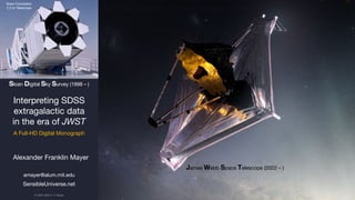
  • 1. Alexander Franklin Mayer amayer@alum.mit.edu SensibleUniverse.net Interpreting SDSS extragalactic data in the era of JWST A Full-HD Digital Monograph James Webb Space Telescope (2022 – ) Sloan Foundation 2.5 m Telescope Sloan Digital Sky Survey (1998 – ) © 2023–2024 A. F. Mayer Study each page with care and attention to detail.
  • 2. 📄 Table of Contents 2 Review of the canonical cosmological model ..………………………………………………………………………………… 3 JWST observations………………………………………………………………………………………………………………… 7 Predictive models confronted by empirical data (6-page preview) .……………………………………………………… 12 MAGIC23 conference abstract @cern.ch.……………………………………………………………………………………… 18 Two predictive cosmological models…………………………………………………………………………………………… 19 The Sloan Digital Sky Survey (SDSS)…………………………………………………………………………………………… 24 SDSS theta-z data………………………………………………………………………………………………………………… 27 The new cosmological model….………………………………………………………………………………………………… 72 Space-density of active galactic nuclei (NED AGN) ..………………………………………………………………………… 76 SDSS, 2dF, and NED AGN data suggest fractal cosmic architecture.……………………………………………………… 85 2dF Galaxy Redshift Survey blueshifts.………………………………………………………………………………………… 92 SDSS Petrosian magnitudes (redshift-magnitude data) ……………………………………………………………………… 93 Summary .………………………………………………………………………………………………………………………… 101 ‘Dark matter’……………………………………………………………………………………………………………………… 107 Quotes .…………………………………………………………………………………………………………………………… 108 The Astrophysical Journal (ApJ)..……………………………………………………………………………………………… 111 Reproducibility…………………………………………………………………………………………………………………… 112 This is a dynamic document; click here for version check. page # v 2024-04-09-00z amayer@alum.mit.edu • SensibleUniverse.net This blue is reserved for clickable 🔗. Magenta is reserved for annotations. A links icon on any graphic denotes an associated link. This document has 200+ Internet links. Links are retrieved using 4ref.de 🐶 🔗 Study each page with care and attention to detail. 64
  • 3. • The most fundamental assumption of the Big Bang theory is that the observed cosmological redshift of galaxies is caused by the uniform expansion of space. • Such an expansion would cause the space between galaxies to increase over time, which corresponds to a modeled general recessional velocity between galaxies. • The wavelength of a receding light source is broadened towards the red end of the visible spectrum in proportion to recession velocity, and similarly by the modeled uniform expansion of space during light propagation; redshift is a dimensionless quantity designated by z that is applicable to photons of any source wavelength. • In a uniformly-expanding medium, each unit of distance expands at the same rate, thus the recessional velocity between points is directly proportional to distance; doubling the distance between points corresponds to doubling their relative velocity. • Light travels at a fi nite speed; galaxies observed at greater distance (higher z) are observed at greater lookback time, or farther back on the modeled cosmic timeline from the current ‘age of the Universe’ back to the origin of that timeline at T = 0. • If we reverse the modeled expansion, then all of the galaxies occupy a volume of space that becomes smaller and smaller over time, culminating in a hot and dense ‘singularity’ of space and time that Sir Fred Hoyle fl ippantly dubbed the “Big Bang”. 3 ⎧ ⎪ ⎨ ⎪ ⎩ details next 3 pages ca•non•i•cal (adjective) : according to recognized rules or scienti fi c laws [historically, often found in need of correction]. Gyr : 1 billion (109) years Gly : 1 billion (109) light years or ~1022 km … amayer@alum.mit.edu • SensibleUniverse.net © 2023 A. F. Mayer The canonical uniform cosmic expansion — fundamentals
  • 4. The canonical uniform cosmic expansion (A) 4 Source of the canonical numerical values: Ned Wright’s Javascript Cosmology Calculator •L and N are equidistant from M, and the distance L–N is 2d. •L and M mutually recede at speed v. •N and M mutually recede at speed v. •L and N mutually recede at speed 2v. d ↔︎ v , 2d ↔︎ 2v , 3d ↔︎ 3v … nd ↔︎ nv v = H0·d v 2d M L N d = a ∙ DC d Big Bang light travel time (Gyr) comoving distance (Gly) Observer—Now 13.2 30.7 12.8 27.5 10.4 17.2 12.2 23.9 7.8 10.9 5.8 7.3 2.5 2.7 4.3 5.1 1.3 1.4 13.7 46.4 0 0 0 ∞ scale factor (1 + z)–1 0.50 1 0.33 2 0.20 4 0.14 6 0.91 0.1 0.83 0.2 0.71 0.4 0.63 0.6 1 0 a z t DC 13.3 32.8 0.08 12 0.10 9 The scale factor (a) is the cosmic radius (i.e., the ‘size of the Universe’) relative to ‘now’ (1). The light travel time (t) is the di ff erence between the cosmic age ‘now’ and age at z. The comoving distance DC (z) to a particular object has a fi xed value over time, similar to the angle between two points on the surface of an inflating ball. The proper distance in a particular epoch is d = a ∙ DC , so d and DC are equivalent ‘now’, and the proper distance between galaxies at z > 12 was considerably less than 1/10th of current values. The Hubble constant (H0) is the current-epoch (a = 1) rate of expansion, typically measured in km/s/Mpc. © 2023 A. F. Mayer amayer@alum.mit.edu • SensibleUniverse.net H0 = 69.6 km·s–1·Mpc–1 ≈ 0.07c·Gly–1 ΩM = 0.286 ΩΛ = 0.714 redshift (z) ⎧ ⎨ ⎩ 2v ⎧ ⎨ ⎩
  • 5. The canonical uniform cosmic expansion (B) 5 © 2023 A. F. Mayer amayer@alum.mit.edu • SensibleUniverse.net BB! 1. JWST observes a GALAXY at z = 9; it has fi xed coordinate DC ≈ 30.7 Gly. 2. We observe that GALAXY as it existed t ≈ 13.2 Gyr years ago (i.e., in our distant past). 3. At that time, the age of the Universe (i.e., the time since the Big Bang) was about 550 Myr (T ≈ 0.55 Gyr). 4. At that time, the Universe was 1/10th (a = 0.1) the current size. 5. At that time, its distance from the Milky Way was d = a·DC ≈ 3.1 Gly. 6. Due to cosmic expansion, its light ‘chased’ the receding Milky Way… 7. and it took t ≈ 13.2 Gyr for that light to arrive at the JWST telescope. 8. At the current age of the cosmos (T ≈ 13.7 Gyr), that GALAXY is now at a distance of d = a·DC ≈ 30.7 Gly and receding at superluminal velocity (v > c). JWST ~30.7 z = 9 GALAXY now z = 0 z = 0.3 z = 1 9 a = 1 a = 0.5 0.1 a ≈ 0.77 d = a · D C ≈ 3 0 . 7 Milky Way DC ≈ 10.9 DC ≈ 3.9 DC = 0 ~0.55 T ≈ 5.9 T ≈ 10.3 T ≈ 13.7 d = a · 3 0 . 7 ≈ 2 3 . 6 d ≈ 1 5 . 4 ~ 3 . 1 t = 0 t ≈ 3.4 t ≈ 7.8 ~13.2 Milky Way 🕰 z : redshift a : scale factor DC : comoving distance (Gly) d : proper distance (Gly) T : cosmic age (Gyr) t : light travel time (Gyr) “lookback” In fl ationary epoch 10−36 ≲ T ≲ 10−32 sec Δa ~ 1026 Source of the canonical numerical values: Ned Wright’s Javascript Cosmology Calculator BB! VIEW ANIMATION 13.2 Gly (Gyr · c) H0 = 69.6 km·s–1·Mpc–1 ≈ 0.07c·Gly–1 ΩM = 0.286 ΩΛ = 0.714 BB!
  • 6. The canonical cosmic timeline • From 2014–2022, the “1% Concordance” model (H0 = 69.6 ± 0.7, ΩM = 0.286, ΩΛ = 0.714) gave the much-publicized, and ostensibly well-established ‘age of the Universe’ to be about 13.7 billion years, the value that most people today were either taught in school, read about in a magazine, or saw in a television program or Internet science video. • According to the latest (2022) reported “precise measurement” of the Hubble constant (H0 = 73.30 ± 1.04) and “a consensus ΛCDM with ΩM = 0.3 and ΩΛ = 0.7”, the modeled age of the Universe ✴︎ since the singularity has been revised, being reduced to ~12.9 Gyr. • The ΛCDM model with the foregoing parameters correlates the measured redshift of a galaxy (z) with the modeled age of the Universe in billions of years (T) at that redshift: 6 Big Bang Canonical age of the Universe (Gyr) ▪︎ [1% Concordance model] 0.94 0.87 3.32 3.08 1.56 1.45 5.90 5.49 7.94 7.40 11.27 10.53 9.40 8.77 12.41 11.61 13.72 12.86 0 ∞ 0.50 1 0.33 2 0.20 4 0.14 6 0.91 0.1 0.83 0.2 0.71 0.4 0.63 0.6 1 0 a z 0 0 T 0.37 0.35 0.08 12 JWST is observing galaxies at z > 12… 0.55 0.51 0.10 9 H0 = 69.6 ΩM = 0.286 ΩΛ = 0.714 H0 = 73.30 ΩM = 0.3 ΩΛ = 0.7 JWST © 2023 A. F. Mayer amayer@alum.mit.edu • SensibleUniverse.net Now Source of the canonical numerical values: Ned Wright’s Javascript Cosmology Calculator redshift (z) scale factor (1 + z)–1 ✴ But NOW, a new published claim [MNRAS (7 July 2023)] is 27.7 Gyr! 🤨
  • 7. 7 Blue Dot — Section Mark & Return to Table of Contents • Companion paper: . “Surveys with James Webb Space Telescope (JWST) have discovered candidate galaxies in the first 400 Myr of cosmic time. … Here we identify four galaxies located in the JWST Advanced Deep Extragalactic Survey Near-Infrared Camera imaging with photometric redshifts z of roughly 10–13. These galaxies include the first redshift z > 12 systems discovered with distances spectroscopically confirmed by JWST in a companion paper.” B. E. Robertson, S. Tacchella, B. D. Johnson, K. Hainline, L. Whitler et al., “Identi fi cation and properties of intense star-forming galaxies at redshifts z > 10”, Nat Astron (4 April 2023). Emma Curtis-Lake et al., Nat Astron (4 April 2023)
  • 8. 8 Fulvio Melina, “The Cosmic Timeline Implied by the JWST High-redshift Galaxies”, arXiv:2302.10103 [astro-ph.CO] (20 Feb 2023). “The so-called ‘impossibly early galaxy’ problem, first identified via the Hubble Space Telescope’s observation of galaxies at redshifts z > 10, appears to have been exacerbated by the more recent James Webb Space Telescope (JWST) discovery of galaxy candidates at even higher redshifts (z ~ 17) which, however, are yet to be confirmed spectroscopically. These candidates would have emerged only ~ 230 million years after the big bang in the context of ΛCDM, requiring a more rapid star formation in the earliest galaxies than appears to be permitted by simulations adopting the concordance model parameters. This time-compression problem would therefore be inconsistent with the age-redshift relation predicted by ΛCDM.”
  • 10. 10 “Deep space observations of the JWST have revealed that the structure and masses of very early Universe galaxies at high redshifts (z ∼ 15), existing at ∼0.3 Gyr after the Big Bang, may be as evolved as the galaxies in existence for ∼ 10 Gyr. The JWST findings are thus in strong tension with the ΛCDM cosmological model. While tired light (TL) models have been shown to comply with the JWST angular galaxy size data, they cannot satisfactorily explain isotropy of the cosmic microwave background (CMB) observations or fit the supernovae distance modulus versus redshift data well. We have developed hybrid models that include the tired light concept in the expanding universe. The hybrid ΛCDM model fits the supernovae type 1a data well but not the JWST observations. …” Ivo Labbé, Pieter van Dokkum, Erica Nelson, Rachel Bezanson, Katherine A. Suess et al., “A population of red candidate massive galaxies ~600 Myr after the Big Bang”, Nature (22 Feb 2023); https://doi.org/10.1038/s41586-023-05786-2. Also see: Michael Boylan-Kolchin, Nat Astron (13 April 2023). Rajendra P Gupta, “JWST early Universe observations and ΛCDM cosmology”, MNRAS (7 Jul 2023); https://doi.org/10.1093/mnras/stad2032.
  • 11. 1-min video James Webb Space Telescope (JWST) Something is amiss; the distant Universe (z ~ 10) apparently contains big, mature galaxies, where only “baby” galaxies are predicted to exist so soon after T = 0. JWST observations clearly put the ΛCDM standard model of Big Bang cosmology in jeopardy; has the model indeed failed? Image credit: NASA (Artist Impression) 11 First data release 12 July 2022 Throughout this monograph: Focal points appear in magenta. Internet links appear in light blue. Follow the data & no winking… amayer@alum.mit.edu • SensibleUniverse.net webb.nasa.gov ‘While Hubble currently has the ability to peer billions of years into the past to see “toddler” galaxies, the JWST will have the capability to study “baby” galaxies, the fi rst galaxies that formed in the Universe.’ – esa potw1819a (7 May 2018) 😉 (references the controversial 2 Sept. 2023 NYT article)
  • 12. Each model† is based on a distinct, known exact solution of the Einstein field equations. Model A: Einstein (1917) → ΛCDM model Model B: de Sitter (1917) → ‘RTG’* model Gμν + Λgμν = κTμν 12 amayer@alum.mit.edu • SensibleUniverse.net We will compare the predictive accuracy of two competing cosmological models. General Audience: Ignore the unintelligible equations—they don’t matter to you; they are like a foreign language (外語), and it is perfectly OK that you don’t know it. * Relativistic Temporal Geometry, motivated by Minkowski (1909). Pages 13 – 17 preview that comparison. † The three new ‘RTG’ predictive formulas are a logically consistent set (i.e., any one formula can be true if and only if all three formulas are true). • 🔗 🔗 🔗 🔗
  • 13. 0:005 0:01 0:02 0:03 0:04 0:05 0:1 0:2 0:3 0:4 0:5 1 SpecPhoto:z (redshift) 0:2 0:3 0:4 0:5 1 2 3 4 5 10 20 30 Galaxy: petroR50 gri (half-light radius 3-band average in arcsec) ΛCDM predictive curves 13 0.32 0.08 0.02 amayer@alum.mit.edu • SensibleUniverse.net • Data: SDSS smallest galaxies 10× reference petroR50_gri --- ΛCDM curves H0 = 69.6 ΩM = 0.286 ΩΛ = 0.714 “theta = size / DA” --- θ ̅z data As per di ff erences in ‘measurements’ of (H0, ΩM, ΩΛ), such variation has no appreciable e ff ect on these curves. intercept 62← ⎧ ⎪ ⎨ ⎪ ⎩ Wright (2006) ~2.4M measurements Empirical reference curve (constant intrinsic-galaxy-size as per linear fi t to data points) The data does not support the model; the ΛCDM model fails catastrophically.* *This model is irreconcilable with the data. z-bin Apparent size vs. redshift
  • 14. 0:005 0:01 0:02 0:03 0:04 0:05 0:1 0:2 0:3 0:4 0:5 1 SpecPhoto:z (redshift) 0:2 0:3 0:4 0:5 1 2 3 4 5 10 20 30 Galaxy: petroR50 gri (half-light radius 3-band average in arcsec) petroR50_gri 14 θ(z) = Cℓ ( 1 − 1 (z + 1)2 ) −1 2 , Cℓ = 1 0.32 0.08 0.02 0.64 0.16 0.04 0.01 --- θ(z) --- θ ̅z data amayer@alum.mit.edu • SensibleUniverse.net • Data: SDSS There are no free parameters to modify the curve; Cℓ merely shifts the curve up or down on the θ-axis. (remarkably, not an arbitrary #) The RTG predictive model fi ts the data. Cℓ = 2 Cℓ = 0.5 1 reference constants 69← N = 398 3.5k 8.3k 38.8k 34.7k 36.5k 7.1k Bin galaxies: [constant intrinsic galaxy size] Minimal-data measurement z-bin Apparent size vs. redshift
  • 15. VC(z) N(z) Cumulative AGN count 102 103 104 105 106 109 Comoving volume V C ( VSmoots ) 103 106 109 Redshift (z) 0.01 0.1 1 10 The third and quite certain interpretation of the graph is that this redshift-volume model [VC(z)] is radically unphysical. 3︎⃣ ρAGN 7.40E–5 ΛCDM: over time, AGN space density increases by ~4 orders of magnitude. Another possible interpretation of the graph, is that ≪1% of AGN that exist at higher redshift are observed and counted by the various astronomical surveys. 15 ρAGN 1 ρAGN = N(z) VC(z) ΛCDM Lookback: 140 Myr ΛCDM Lookback: 12.86 Gyr 6.42 H0 = 69.6 ΩM = 0.286 ΩΛ = 0.714 1︎⃣2︎⃣ Δzbin = 0.001 [arbitrary units] The data does not support the model; the ΛCDM model fails catastrophically. amayer@alum.mit.edu • SensibleUniverse.net • Data: NED 81← (for intercept) >4 orders of magnitude! Volume/AGN vs. redshift ΛCDM: cosmic galaxy evolution over ~12.7 Gyr
  • 16. S3 (z) N(z) Cumulative AGN count 102 103 104 105 106 109 Proper volume (arbitrary units) 103 106 109 Redshift (z) 0.01 0.1 1 10 S3 (z) = CV ⋅ cos−1 ( 1 z + 1) − ( 1 (z + 1)2 − 1 (z + 1)4 ) 1 2 S3 represents the volumetric ‘surface’ of a Riemannian 3-sphere The fi t of this a priori theoretical predictive curve to the empirical AGN population data is equally remarkable to that for the theta-z data; there are no free parameters available to achieve this fi t. 16 Δzbin = 0.001 same intercept amayer@alum.mit.edu • SensibleUniverse.net • Data: NED 82← CV = 9.7E4 (sets the intercept) Volume/AGN vs. redshift The RTG predictive model fi ts the data. The interpretation of this graph is that AGN are accurately counted, even out to very high redshift, and that galaxy clusters comprise a fi xed percentage of AGN throughout the Universe.
  • 17. intercepts (0.32, 18.2) (0.32, 16.6) Redshift-magnitude curves modeling constant intrinsic brightness 17 Note: g-band data must exhibit 4000 Å break! Data: ~136k SDSS LRGs (z-band) RTG: m(z) = CM − 2.5 log [ 1 4π ((z + 1)4 − (z + 1)2 ) ] + ϵλ ⋅ cos−1 ( 1 z + 1) − CM = 14.82, 13.22 ϵλ = 0.5 CM = 15.17, 13.57 ϵλ = 0 − − ΛCDM: m(z) = KM − 2.5 log [ 1 4πD2 L ] − KM = − 0.68, − 2.28 amayer@alum.mit.edu • SensibleUniverse.net • Data: SDSS 97← The SDSS Luminous Red Galaxies (LRGs) were speci fi cally selected to have similar characteristics, including their luminosity. extinction RTG constant-intrinsic-brightness model The RTG predictive model fi ts the data. ΛCDM constant-intrinsic-brightness model The data does not support this model.* * The ΛCDM model fails catastrophically.
  • 18. https://indico.cern.ch/event/1153372/contributions/5200955/ 18 “Facts do not cease to exist because they are ignored.” – Aldous Huxley (1927) • of ~ 🔗 End of preview; Main Presentation • ⤺Table of Contents What is Science? (2-minute video)
  • 19. – Yuri Ivanovich Manin, Talk on Computability, Northwestern University (c. 1995) “When I was starting out in mathematics, it seemed very important to prove a big theorem. Now, with more experience, I understand that it is new notions that are more important, for example, Alan Turing’s new notion of computability, which I shall discuss today.” 19 amayer@alum.mit.edu • SensibleUniverse.net I thank Dr. Michael Stephen Fiske, Ph.D. Mathematics, Northwestern (1996) for this quotation. • As per this quote that Dr. Fiske had previously shared with me, I contacted Yuri, and he then invited me to meet with him at his o ffi ce at the Max-Planck-Institut für Mathematik in Bonn on 14 August 2009. We spoke about mathematical physics in a cordial discussion of well over two hours in which I fi lled three whiteboards with equations and diagrams. Our discussion concluded with Yuri memorably re fl ecting on the fact that his contributions to fi eld theory represented a signi fi cant lifetime investment — read between the lines. Best Paper Award HICSS 2022 & 2023
  • 20. ψ ψ 20 Spherical coordinate system (r, θ, ψ) amayer@alum.mit.edu • SensibleUniverse.net The following page (21) presents Einstein’s 1917 exact solution of the fi eld equations in the form of a metric (i.e., an equation that measures distance). It is important to understand that the locally-de fi ned blue vector r here is the same dimension of physical space as the blue arc r on page 21, and that the dot at the origin here can represent any point on the circle. The interior region of the blue circle of radius R does not represent space; the other two space dimensions (θ, ψ), over which distances between galaxies can be measured, are not represented in the diagram. We call the Euclidean coordinate system on the left, which represents strictly-locally-de fi ned measurable 3-dimensional physical space, a tangent space. Each such tangent space has a 4th coordinate, t that represents time as locally measured in that space; t is mutually orthogonal to the three space coordinates in accord with the locally-applicable Minkowski metric. ds2 = x2 + y2 + z2 + (ict)2 local Minkowski metric Note that i2 = –1 This Euclidean coordinate system is valid only in the neighbourhood of its own origin at r = 0. page-21 preview r R s p a ce Milky Way Distant Galaxy
  • 21. Model (“System”) A Einstein’s metric —an exact solution of the Einstein fi eld equations (EFE) 21 t r R Riemannian geometry vs. Euclidean geometry amayer@alum.mit.edu • SensibleUniverse.net ✓ R ∝ a (dimensionless cosmic scale factor) The blue circle represents a cosmological great circle — a single dimension of measurable physical space in two dimensions of ℝ4. ℝ4 means a 4D Euclidean space, which may contain a 4-dimensional sphere. ds2 = − dr2 − R2 sin2 ( r R) [dψ2 + sin2 (ψ) dθ2 ] + c2 dt2 dθ = dΨ = 0 χ ≡ r R χ ∝ DC χ © 2023 A. F. Mayer A. Einstein, “Cosmological Considerations in the General Theory of Relativity”, SPAW, 142 (1917). ✓ 1) The Universe is fi nite, yet has no boundary. 2) Time is independent of space in the metric. equivalence proportionality 58← & symmetry! s p a ce 1-minute VIDEO Milky Way Distant Galaxy
  • 22. – Willem de Sitter (31 March 1917) “We thus find that in the System A the time has a separate position. That this must be so, is evident a priori. For speaking of the three- dimensional world, if not equivalent to introducing an absolute time, at least implies the hypothesis that at each point of the four-dimensional space there is one absolute coordinate x4 which is preferable to all others to be used as “time”, and that at all points and always this one coordinate is actually chosen as time. Such a fundamental difference between the time and the space-coordinates seems to be somewhat contradictory to the complete symmetry of the field-equations…” W. de Sitter, “On the relativity of inertia. Remarks concerning Einstein’s latest hypothesis”, KNAW Proceedings 19(2), 1217 (1917). 22 amayer@alum.mit.edu • SensibleUniverse.net Referencing Einstein’s metric, expressed using x4 ≡ t ⎫ ⎪ ⎬ ⎪ ⎭
  • 23. W. de Sitter, “Einstein’s theory of gravitation and its astronomical consequences. Third paper”, MNRAS 78, 3 (1917). Model B Willem de Sitter’s metric — a different exact solution of the EFE 23 This interpretation of de Sitter’s metric, where time is a strictly-local geometric object is new. It also elegantly resolves the quandary of zero cosmic matter density imposed by this solution. amayer@alum.mit.edu • SensibleUniverse.net dρ2 = − dρ1 ∴ ∫ 2π 0 dρ = ρ = 0 Cosmic perspective relativistic perspective density ds2 = − dr2 − R2 sin2 ( r R) [dψ2 + sin2 (ψ) dθ2 ] + cos2 ( r R ) c2 dt2 c2dτ2 locally dρ1 > 0 locally dρ2 > 0 dρn is local mass-energy density t τ r R 1 2 cos ( r R) = cos χ = dτ dt energetic relationship → 1) The Universe is fi nite, yet has no boundary. 2) Time is dependent on space in the metric. © 2023 A. F. Mayer 65← · R = 0 χ dθ = dΨ = 0 χ ≡ r R
  • 24. “In 1987 Gunn proposed putting an array of CCDs on a 2.5m-telescope…” J. E. GUNN ET AL., “The 2.5 m Telescope of the Sloan Digital Sky Survey”, The Astronomical Journal, 131:2332–2359, 2006 April. 24 Creative Innovator & Leader PRINCETON UNIVERSITY Adapted from a screen shot of Gunn’s o ffi cial web page at Princeton. •
  • 25. photo credit: Reidar Hahn, Fermilab Visual Media Services Sloan Foundation 2.5-m Telescope Sloan Digital Sky Survey SDSS.org 25
  • 26. Apache Point Observatory Sunspot, New Mexico, USA 26
  • 27. “The core of science is not mathematical modeling; it is intellectual honesty. It is a willingness to have our certainties about the world constrained by good evidence and good argument.” ⋮ “Either a person is being intellectually honest, or he isn’t. Either a person is willing to look dispassionately at the data or he is trying to conform the data to his prior conception of the world. And science, when it is working, which is to say when it is really science, amounts to a systematic eschewal of dogma. I mean, dogma in science is humiliating, whenever it is recognized to be dogma.” – Sam Harris Beyond Belief: Science, Reason, Religion & Survival, Salk Institute (Nov 2006) Also appearing at the conference, Neil deGrasse Tyson amayer@alum.mit.edu • SensibleUniverse.net 🌱 ⚰ Theories live and die by accurate empirical data. 27 • ac·cu·rate (adjective) : faithfully or fairly representing the truth about someone or something. “Scientists are more readily bought than politicians.” – anon.
  • 29. 0:005 0:01 0:02 0:03 0:04 0:05 0:1 0:2 0:3 0:4 0:5 1 SpecPhoto:z (redshift) 0:2 0:3 0:4 0:5 1 2 3 4 5 10 20 30 Galaxy: petroR50 gri (half-light radius 3-band average in arcsec) BLUE DOT REPRESENTS ONE GALAXY BLUE: sparser data → RED: denser data Theta-z log-log plot of half-light radius (petroR50) for ~800k galaxies Measured apparent radius (arcsec) 29 Low-z ⬅︎ NEARER High-z FARTHER ➡︎ SMALLER ⇩ ⇧ LARGER z = 0.32 z = 0.08 z = 0.02 z = 1 z = 0.01 Theta-z ≡ “apparent size versus redshift” amayer@alum.mit.edu • SensibleUniverse.net • Data: SDSS Color scaling is log2. Blue dot 1 galaxy Cyan dot 2 galaxies Yellow dot 4 galaxies Red dot 8 galaxies
  • 30. Source: Glossary of SDSS-IV Terminology SDSS glossary reference petroRad The Petrosian radius. A measure of the angular size of an image, most meaningful for galaxies. Units are seconds of arc. The Petrosian radius (and related measures of size called petroR50 and petroR90) are derived from the surface brightness profile of the galaxy, as described in Algorithms. Surface Brightness The frames pipeline also reports the radii containing 50% and 90% of the Petrosian flux for each band, petroR50 and petroR90 respectively. … 30
  • 31. Understanding SDSS angular resolution (“theta” measurement) Average apparent diameter of full Moon at zenith: 31.6′ = 1896ʺ. Compared relative to the average apparent size of the full Moon, the green dot has a 10ʺ diameter; that same size is also compared to a z ~ 0.08 SDSS galaxy. 31 © 2016–2023 A. F. Mayer Click image for SDSS SkyServer Explorer. 10ʺ ObjID: 1237658298990330048 petroRad_gri = 18.5±0.3ʺ Petrosian radius ∴ petroRad circle encloses ~7k CCD pixels – petroR50 circle encloses ~2k CCD pixels rP petroR50_gri = 9.8±0.1ʺ half-light radius z = 0.0762 0.396 arcsec∙pix–1 OPTICAL NEGATIVE amayer@alum.mit.edu • SensibleUniverse.net 🌎 Apogee (29.9′ ) Perigee (33.5′ ) Semimajor axis (31.6′ ) Earth-Moon System to scale green dot 🔗
  • 32. Reference: r The observed radial galaxy brightness pro fi le [ I(r′) ] is “azimuthally averaged” (i.e., averaged over 2π radians). ≡ d ′ r 2π ′ r I ′ r ( )/ π 1.252 − 0.82 ( )r2 0.8r 1.25r ∫ d ′ r 2π ′ r I ′ r ( )/ πr2 0 r ∫ 𝓡 P(r) local surface brightness in annulus (blue region) 0.8r r 1.25r Here, r is a variable measurement; it is not a recorded measurement. DEFINITION: “Petrosian ratio” [ 𝓡 P(r)] 1.25r 0.8r mean surface brightness measured inside radius r ÷ Define 𝓡 P,lim as 𝓡 P(rP) = 𝓡 P,lim where rP is the measured and recorded Petrosian radius. 𝓡 P,lim = 0.2 for the SDSS: Varying r, when 𝓡 P(r) = 0.2, then rP = r. Petrosian radius (SDSS “petroRad” measurement) 32 © 2015–2023 A. F. Mayer amayer@alum.mit.edu • SensibleUniverse.net 𝓡 P(r) ≡ Measures Of Flux And Magnitude – Petrosian Magnitudes: petroMag
  • 33. 0:005 0:01 0:02 0:03 0:04 0:05 0:1 0:2 0:3 0:4 0:5 1 SpecPhoto:z (redshift) 0:2 0:3 0:4 0:5 1 2 3 4 5 10 20 30 Galaxy: petroR50 gri (half-light radius 3-band average in arcsec) ObjID: 1237658298990330048 33 SDSS 18 finding chart Every galaxy plotted includes this basic empirical data and far more. Click for more data… theta-z coordinates of this galaxy (petroR50_gri) OPTICAL NEGATIVE amayer@alum.mit.edu • SensibleUniverse.net • Data: SDSS SDSS SkyServer Database Values (arcsec) petroRad_g 18.22892±0.27 petroRad_r 18.69740±0.31 petroRad_i 18.64179±0.35 petroRad_gri 18.52±0.31 petroR50_g 9.70912±0.11 petroR50_r 9.77527±0.06 petroR50_i 9.83906±0.05 petroR50_gri 9.77±0.08 z 0.076242 zErr 2.46E-05 🔗
  • 34. Ultraviolet u Green g Red r Near Infrared i Infrared z 3531 4627 6140 7467 8887 Central wavelengths λeff (Å) from Doi et al. (2010),Table 2. SDSS astronomical band-pass fi lters λeff (Å) Not redshift (z)! photo credit: Michael Carr photo credit: Smithsonian National Air and Space Museum 34 disambiguation for a general audience Click for article… amayer@alum.mit.edu • SensibleUniverse.net 🔗
  • 35. 0:005 0:01 0:02 0:03 0:04 0:05 0:1 0:2 0:3 0:4 0:5 1 SpecPhoto:z (redshift) 0:2 0:3 0:4 0:5 1 2 3 4 5 10 20 30 Galaxy: petroR50 gri (half-light radius 3-band average in arcsec) ~2.4×10⁶ Empirical Measurements 35 ~2.4 MILLION measurements There are 795,838 galaxies (data) represented in this graph, and each datum represents the average of 3 distinct (g, r, i) radius measurements. Too many measurements to “massage” the data according to con fi rmation bias. 0.32 1 0.08 0.02 0.01 amayer@alum.mit.edu • SensibleUniverse.net • Data: SDSS Apparent size vs. redshift
  • 36. 0:005 0:01 0:02 0:03 0:04 0:05 0:1 0:2 0:3 0:4 0:5 1 SpecPhoto:z (redshift) 0:2 0:3 0:4 0:5 1 2 3 4 5 10 20 30 Galaxy: petroR50 gri (half-light radius 3-band average in arcsec) 36 smallest galaxies 10× reference petroR50_gri 0.32 1 0.08 0.02 0.01 SDSS cannot see the smallest galaxies at this great distance. Far away, the faint outer regions of the largest galaxies are not seen, so they appear smaller. Galaxies at the peak of each reference rod are 10× greater in measured radius than those at the base. amayer@alum.mit.edu • SensibleUniverse.net • Data: SDSS
  • 37. The intrinsic radial size of typical galaxies, including all morphologies, spans an order of magnitude (i.e., ×10), which decadal range excludes statistically-unlikely outliers. ① 37 Empirical Inference Inference | ˈinf(ə)rəns | noun a conclusion reached on the basis of evidence and reasoning: researchers are entrusted with drawing inferences from the data. amayer@alum.mit.edu • SensibleUniverse.net
  • 38. 0:005 0:01 0:02 0:03 0:04 0:05 0:1 0:2 0:3 0:4 0:5 1 SpecPhoto:z (redshift) 0:2 0:3 0:4 0:5 1 2 3 4 5 10 20 30 Galaxy: petroR50 gri (half-light radius 3-band average in arcsec) 38 ×2 ×2 ×2 ×2 ×2 ×2 7 Redshift (z ̅) Bins Each bin allows us to examine a group of galaxies that are close to each other in redshift (i.e., at about the same distance). amayer@alum.mit.edu • SensibleUniverse.net • Data: SDSS 0.01 0.02 0.04 0.08 0.16 0.32 0.64 z ̅ = 398 3.5k 8.3k 38.8k 34.7k 36.5k 7.1k N ≊ galaxy count average redshift
  • 39. 0:0760 0:0765 0:0770 0:0775 0:0780 0:0785 0:0790 0:0795 0:0800 0:0805 0:0810 0:0815 0:0820 0:0825 0:0830 0:0835 0:0840 SpecPhoto:z (redshift) 1 2 3 4 5 10 Galaxy: petroR50 gri (half-light radius 3-band average in arcsec) 39 Measurement-error ellipses for z ̅ = 0.080 (5% regular sample of the bin) 0.760 0.084 0.080 Measured apparent radius (arcsec) Redshift (z) nth selection sample interval = 20 amayer@alum.mit.edu • SensibleUniverse.net • Data: SDSS
  • 40. 0:304 0:306 0:308 0:310 0:312 0:314 0:316 0:318 0:320 0:322 0:324 0:326 0:328 0:330 0:332 0:334 0:336 SpecPhoto:z (redshift) 1 2 3 4 5 10 Galaxy: petroR50 gri (half-light radius 3-band average in arcsec) 40 0.304 0.336 0.320 Measurement-error ellipses for z ̅ = 0.320 (5% regular sample of the bin) nth selection sample interval = 20 amayer@alum.mit.edu • SensibleUniverse.net • Data: SDSS
  • 41. 0:005 0:01 0:02 0:03 0:04 0:05 0:1 0:2 0:3 0:4 0:5 1 SpecPhoto:z (redshift) 0:2 0:3 0:4 0:5 1 2 3 4 5 10 20 %petroR50Err gri (radius measurement error as a % of measurement) Radius measurement error (petroR50Err) as a percent of the measurement 41 20% pop. at z ≥ 0.310 80% pop. 10% 5% 1% Error % 1 0.08 0.02 0.01 0.32 amayer@alum.mit.edu • SensibleUniverse.net • Data: SDSS
  • 42. 0:005 0:01 0:02 0:03 0:04 0:05 0:1 0:2 0:3 0:4 0:5 1 SpecPhoto:z (redshift) 0:2 0:3 0:4 0:5 1 2 3 4 5 10 20 30 Galaxy: petroR50 gri (half-light radius 3-band average in arcsec) A Massive Volume of High-Quality Data Principle galaxy selection criteria: •Maximum allowed radius-measurement error in any of the three bands is 20%. •Maximum allowed redshift error is 1%. Plotted theta-z data set: •Average gri radius-measurement error is 3.6%. •Average redshift-measurement error is 0.021%. 42 amayer@alum.mit.edu • SensibleUniverse.net
  • 43. 0:005 0:01 0:02 0:03 0:04 0:05 0:1 0:2 0:3 0:4 0:5 1 SpecPhoto:z (redshift) 0:2 0:3 0:4 0:5 1 2 3 4 5 10 20 30 Galaxy: petroR50 gri (half-light radius 3-band average in arcsec) ✓ Minimum Redshift zmin Maximum Redshift zmax Average Redshift Galaxy count N StdDev[ ln(r) ] σ ln(r) µ Mean Radius Median Radius Standard Deviation 0.0090 0.0110 0.010 398 0.6711 1.5170 5.71 4.56 1.96 0.0180 0.0220 0.020 3,483 0.5593 1.3984 4.73 4.05 1.75 0.0380 0.0420 0.040 8,345 0.4686 1.1179 3.41 3.06 1.60 0.0760 0.0840 0.080 38,831 0.3870 0.8200 2.45 2.27 1.47 0.1520 0.1680 0.160 34,762 0.2952 0.7156 2.14 2.05 1.34 0.3040 0.3360 0.320 36,487 0.2297 0.4503 1.61 1.57 1.26 0.6100 0.6780 0.640 7,147 0.2236 0.1637 1.21 1.18 1.25 θ = e(μ+σ2 2 ) z = ∑ z ÷ N eμ eσ 43 log-normal distribution Redshift Bin Statistics for petroR50_gri (Geometric vs. Arithmetic) normal distribution✗ amayer@alum.mit.edu • SensibleUniverse.net • Data: SDSS
  • 44. Bin Count (galaxies) Median Radius (4.56) Mean Radius (5.71) Radius-Bin Count (n) 0 5 10 15 20 Galaxy.petroR50_gri (arcsec) 0.5 1 2 5 10 20 Empirical Galaxy-Size Distribution Not much useful data here at low-redshift… 😰 44 0:005 0:01 0:02 0:03 0:04 0:05 0:1 0:2 0:3 0:4 0:5 1 SpecPhoto:z (redshift) 0:2 0:3 0:4 0:5 1 2 3 4 5 10 20 30 Galaxy: petroR50 gri (half-light radius 3-band average in arcsec) amayer@alum.mit.edu • SensibleUniverse.net z ̅ = 0.010 N = 398 ( ∑n ) Δrbin = 0.1″ NOTE: This redshift (0.010) is 3 times greater than the maximum z in Edwin Hubble’s 1929 diagram.
  • 45. 45 NO WORRIES, SDSS HAS AN EXCELLENT TELESCOPE AND A TEAM OF OUTSTANDING ASTRONOMERS… 😎 photo credit: Reidar Hahn, Fermilab Visual Media Services
  • 46. μ = 1.3984 σ = 0.5593 S = 350 (scaling constant) Bin Count (galaxies) Median Radius (4.05) Mean Radius (4.73) PDF*: fX(r; μ, σ) ⋅ S Radius-Bin Count (n) 0 50 100 150 200 Galaxy.petroR50_gri (arcsec) 0.5 1 2 5 10 20 * Probability Density Function Note: the vertical scale is >10× the z ̅ = 0.010 scale. 46 N = 3,483 ( ∑n ) Empirical Galaxy-Size Distribution vs. Analytic Log-Normal Distribution Curve 0:005 0:01 0:02 0:03 0:04 0:05 0:1 0:2 0:3 0:4 0:5 1 SpecPhoto:z (redshift) 0:2 0:3 0:4 0:5 1 2 3 4 5 10 20 30 Galaxy: petroR50 gri (half-light radius 3-band average in arcsec) z ̅ = 0.020 fX(r; μ, σ) = 1 rσ 2π exp − (ln r − μ) 2 2σ2 Δrbin = 0.1″ amayer@alum.mit.edu • SensibleUniverse.net • Data: SDSS
  • 47. μ = 1.1179 σ = 0.4686 S = 800 Bin Count (galaxies) Median Radius (3.06) Mean Radius (3.41) PDF: fX(r; μ, σ) ⋅ S Radius-Bin Count (n) 0 100 200 300 400 Galaxy.petroR50_gri (arcsec) 0.5 1 2 5 10 20 Note: the vertical scale is 2× the z ̅ = 0.020 scale. 47 0:005 0:01 0:02 0:03 0:04 0:05 0:1 0:2 0:3 0:4 0:5 1 SpecPhoto:z (redshift) 0:2 0:3 0:4 0:5 1 2 3 4 5 10 20 30 Galaxy: petroR50 gri (half-light radius 3-band average in arcsec) z ̅ = 0.040 N = 8,345 ( ∑n ) Empirical Galaxy-Size Distribution vs. Analytic Log-Normal Distribution Curve Δrbin = 0.1″ amayer@alum.mit.edu • SensibleUniverse.net • Data: SDSS
  • 48. μ = 0.8200 σ = 0.3870 S = 3850 Bin Count (galaxies) Median Radius (2.27) Mean Radius (2.45) PDF: fX(r; μ, σ) ⋅ S Radius-Bin Count (n) 0 1k 2k 3k 4k Galaxy.petroR50_gri (arcsec) 0.5 1 2 5 10 20 Note: the vertical scale is 10× the z ̅ = 0.040 scale. 48 z ̅ = 0.080 0:005 0:01 0:02 0:03 0:04 0:05 0:1 0:2 0:3 0:4 0:5 1 SpecPhoto:z (redshift) 0:2 0:3 0:4 0:5 1 2 3 4 5 10 20 30 Galaxy: petroR50 gri (half-light radius 3-band average in arcsec) N = 38,831 ( ∑n ) Empirical Galaxy-Size Distribution vs. Analytic Log-Normal Distribution Curve Δrbin = 0.1″ amayer@alum.mit.edu • SensibleUniverse.net • Data: SDSS
  • 49. μ = 0.7156 σ = 0.2952 S = 3700 Bin Count (galaxies) Median Radius (2.05) Mean Radius (2.14) PDF: fX(r; μ, σ) ⋅ S Radius-Bin Count (n) 0 1k 2k 3k 4k Galaxy.petroR50_gri (arcsec) 0.5 1 2 5 10 20 49 z ̅ = 0.160 0:005 0:01 0:02 0:03 0:04 0:05 0:1 0:2 0:3 0:4 0:5 1 SpecPhoto:z (redshift) 0:2 0:3 0:4 0:5 1 2 3 4 5 10 20 30 Galaxy: petroR50 gri (half-light radius 3-band average in arcsec) N = 34,762 ( ∑n ) Note: the vertical scale now remains constant… Empirical Galaxy-Size Distribution vs. Analytic Log-Normal Distribution Curve Δrbin = 0.1″ amayer@alum.mit.edu • SensibleUniverse.net • Data: SDSS
  • 50. μ = 0.4503 σ = 0.2297 S = 3900 Bin Count (galaxies) Median Radius (1.57) Mean Radius (1.61) PDF: fX(r; μ, σ) ⋅ S Radius-Bin Count (n) 0 1k 2k 3k 4k Galaxy.petroR50_gri (arcsec) 0.5 1 2 5 10 20 50 z ̅ = 0.320 0:005 0:01 0:02 0:03 0:04 0:05 0:1 0:2 0:3 0:4 0:5 1 SpecPhoto:z (redshift) 0:2 0:3 0:4 0:5 1 2 3 4 5 10 20 30 Galaxy: petroR50 gri (half-light radius 3-band average in arcsec) N = 36,487 ( ∑n ) Empirical Galaxy-Size Distribution vs. Analytic Log-Normal Distribution Curve Δrbin = 0.1″ amayer@alum.mit.edu • SensibleUniverse.net • Data: SDSS
  • 51. μ = 0.1637 σ = 0.2236 S = 700 Bin Count (galaxies) Median Radius (1.18) Mean Radius (1.21) PDF: fX(r; μ, σ) ⋅ S Radius-Bin Count (n) 0 1k 2k 3k 4k Galaxy.petroR50_gri (arcsec) 0.5 1 2 5 10 20 51 z ̅ = 0.640 0:005 0:01 0:02 0:03 0:04 0:05 0:1 0:2 0:3 0:4 0:5 1 SpecPhoto:z (redshift) 0:2 0:3 0:4 0:5 1 2 3 4 5 10 20 30 Galaxy: petroR50 gri (half-light radius 3-band average in arcsec) N = 7,147 ( ∑n ) Empirical Galaxy-Size Distribution vs. Analytic Log-Normal Distribution Curve Δrbin = 0.1″ amayer@alum.mit.edu • SensibleUniverse.net • Data: SDSS
  • 52. Galaxies have a log-normal size distribution. ② 52 Empirical Inference amayer@alum.mit.edu • SensibleUniverse.net Shiyin Shen, H. J. Mo, Simon D. M. White, Michael R. Blanton, Guinevere Kauffmann et al., “The size distribution of galaxies in the Sloan Digital Sky Survey”, Mon. Not. R. Astron. Soc. 343, 978 (2003). The foregoing analysis generalizes an earlier fi nding dating back two decades:
  • 53. That distribution is empirically observed to be consistent over the data set (0.02 ≤ z ≤ 0.64). ③ 53 Empirical Inference amayer@alum.mit.edu • SensibleUniverse.net
  • 54. To very good approximation, the mean apparent galaxy size (theta-bar) in each redshift bin can be expected to represent the same standard rod (i.e., to be very nearly the same intrinsic size ℓ). ④ 54 Inference | ˈinf(ə)rəns | noun a conclusion reached on the basis of evidence and reasoning: researchers are entrusted with drawing inferences from the data. Empirical Inference amayer@alum.mit.edu • SensibleUniverse.net
  • 55. 0:005 0:01 0:02 0:03 0:04 0:05 0:1 0:2 0:3 0:4 0:5 1 SpecPhoto:z (redshift) 0:2 0:3 0:4 0:5 1 2 3 4 5 10 20 30 Galaxy: petroR50 gri (half-light radius 3-band average in arcsec) 55 Galaxy Mean Radius (θ ̅z) Plotted For Each Redshift Bin (Black Squares) 0.01 0.02 0.04 0.08 0.16 0.32 0.64 z ̅ = amayer@alum.mit.edu • SensibleUniverse.net • Data: SDSS 398 3.5k 8.3k 38.8k 34.7k 36.5k 7.1k N ≊
  • 56. Radius-bin count(n) 0 1000 2000 3000 4000 Galaxy.petroR50_gri (arcsec) 0.6 0.8 1 2 4 6 8 10 12 16 sample galaxy image 56 z = 0.076 z = 0.084 θ ̅ = 2.45″ Δrbin = 0.2″ ObjID: 1237665101141835997 🔗 N = 38,831 galaxies (each dot is a galaxy) bin slice → Color denotes data density; color scaling is log2. z ̅ = 0.08 redshift-bin Δsize = 10 Same data as page 48, but a montage with more detail and di ff erent (×2) Δrbin. 5″ 20″ petroR50_gri 2.450 (120 pix) petroRad_gri 5.124 (526 pix) z 0.0794 petroR50_gri 11.54 ( 2.7k pix) petroRad_gri 28.68 (16.5k pix) z 0.0789 ObjID: 1237678617430589483 🔗 Measurement exaggerated by environs. amayer@alum.mit.edu • SensibleUniverse.net • Data: SDSS 5 extreme outliers ⎧ ⎪ ⎨ ⎪ ⎩ Click image for Skyserver…
  • 57. 0:005 0:01 0:02 0:03 0:04 0:05 0:1 0:2 0:3 0:4 0:5 1 SpecPhoto:z (redshift) 0:2 0:3 0:4 0:5 1 2 3 4 5 10 20 30 Galaxy: petroR50 gri (half-light radius 3-band average in arcsec) Empirical Constant-Intrinsic-Galaxy-Size Curve (linear fi t to θ ̅z data) log θ = − 0.3749 ⋅ log z + 0.01355 --- θ ̅z data Empirical reference curve (constant intrinsic-galaxy-size as per linear fi t to data points) 0.32 0.08 0.02 0.01 1 0.04 0.16 0.64 3× Hubble’s maximum z amayer@alum.mit.edu • SensibleUniverse.net • Data: SDSS Pearson correlation coefficient: – 0.9967 57 (–1 implies a perfect linear relationship.)
  • 58. 58 t Riemannian geometry vs. Euclidean geometry ds2 = − dr2 − R2 sin2 ( r R) [dψ2 + sin2 (ψ) dθ2 ] + c2 dt2 amayer@alum.mit.edu • SensibleUniverse.net A. Einstein, “Cosmological Considerations in the General Theory of Relativity”, SPAW, 142 (1917). ✓ Recall (page 21) Galaxy redshift & time dilation modeled as dR/dt > 0 (i.e., “expanding universe”). r R(t) R ∝ a (dimensionless cosmic scale factor) Model (“System”) A Einstein’s metric —an exact solution of the Einstein fi eld equations (EFE) χ ✓ 1) The Universe is fi nite, yet has no boundary. 2) Time is independent of space in the metric. © 2023 A. F. Mayer dθ = dΨ = 0 χ ≡ r R χ ∝ DC & symmetry! 21→ s p a ce 1-minute VIDEO
  • 59. z = 0.0033 Hubble Diagram (1929) — Annotated E. Hubble, “A Relation between Distance and Radial Velocity among Extra-Galactic Nebulae”, PNAS 15, 168 (1929). Hubble constant modern value* H0 = 69.6 ± 0.7 *Recently updated H0 = 73.30 ± 1.04 (q0 = –0.51 ± 0.024) H0 = 530 amayer@alum.mit.edu • SensibleUniverse.net 59 The historical foundation of the ‘expanding-universe’ paradigm H0 units: km s−1 Mpc −1 H0 = 625 Lemaître (1927) IMPORTANT BACKSTORY HERE D Both H0 values fit the thick blue line.
  • 60. Hubble’s law: v = H0D v ≈ cz (z ≪ 1) “Double the redshift→double the distance.” 60 If this relationship does not hold, the Universe is not expanding. (i.e., model) amayer@alum.mit.edu • SensibleUniverse.net ∴ Double the redshift→half the apparent size.
  • 61. 0:005 0:01 0:02 0:03 0:04 0:05 0:1 0:2 0:3 0:4 0:5 1 SpecPhoto:z (redshift) 0:2 0:3 0:4 0:5 1 2 3 4 5 10 20 30 Galaxy: petroR50 gri (half-light radius 3-band average in arcsec) 61 0.32 0.08 0.02 3× Hubble’s maximum z Hubble’s law predictive curves smallest galaxies 10× reference petroR50_gri --- Hubble’s law --- θ ̅z data (θ ∝ z−1 ) amayer@alum.mit.edu • SensibleUniverse.net • Data: SDSS intercept Empirical reference curve (constant intrinsic-galaxy-size as per linear fi t to data points) Apparent size vs. redshift The data does not support the model; the ‘Hubble law’ fails catastrophically.* *This model is irreconcilable with the data.
  • 62. 0:005 0:01 0:02 0:03 0:04 0:05 0:1 0:2 0:3 0:4 0:5 1 SpecPhoto:z (redshift) 0:2 0:3 0:4 0:5 1 2 3 4 5 10 20 30 Galaxy: petroR50 gri (half-light radius 3-band average in arcsec) ΛCDM predictive curves 62 0.32 0.08 0.02 amayer@alum.mit.edu • SensibleUniverse.net • Data: SDSS smallest galaxies 10× reference petroR50_gri --- ΛCDM curves H0 = 69.6 ΩM = 0.286 ΩΛ = 0.714 “theta = size / DA” --- θ ̅z data As per di ff erences in ‘measurements’ of (H0, ΩM, ΩΛ), such variation has no appreciable e ff ect on these curves. intercept Wright (2006) ~2.4M measurements Empirical reference curve (constant intrinsic-galaxy-size as per linear fi t to data points) 13→ z-bin *This model is irreconcilable with the data. The data does not support the model; the ΛCDM model fails catastrophically.* Apparent size vs. redshift ⎧ ⎪ ⎨ ⎪ ⎩
  • 63. 63 This web page is the authoritative source of the ΛCDM curves. arXiv:astro-ph/9905116v4 16 Dec 2000 Distance measures in cosmology David W. Hogg Institute for Advanced Study, 1 Einstein Drive, Princeton NJ 08540 hogg@ias.edu 2000 December 1 Introduction In cosmology (or to be more specific, cosmography, the measurement of the Universe) there are many ways to specify the distance between two points, because in the expanding Universe, the distances between comoving objects are constantly changing, and Earth-bound observers look back in time as they look out in distance. The unifying aspect is that all distance measures somehow measure the separation between events on radial null trajectories, ie, trajectories of photons which terminate at the observer. In this note, formulae for many different cosmological distance measures are provided. I treat the concept of “distance measure” very liberally, so, for instance, the lookback time and comoving volume are both considered distance measures. The bibliography of source material can be consulted for many of the derivations; this is merely a “cheat sheet.” Minimal C routines (KR) which compute all of these distance measures are available from the author upon request. Comments and corrections are highly appreciated, as are acknowledgments or citation in research that makes use of this summary or the associated code. 2 Cosmographic parameters The Hubble constant H0 is the constant of proportionality between recession speed v and distance d in the expanding Universe; v = H0 d (1) The subscripted “0” refers to the present epoch because in general H changes with time. The dimensions of H0 are inverse time, but it is usually written H0 = 100 h km s−1 Mpc−1 (2) where h is a dimensionless number parameterizing our ignorance. (Word on the street is that 0.6 < h < 0.9.) The inverse of the Hubble constant is the Hubble time tH tH ≡ 1 H0 = 9.78 × 10⁹ h−1 yr = 3.09 × 10¹⁷ h−1 s (3) and the speed of light c times the Hubble time is the Hubble distance DH DH ≡ c H0 = 3000 h−1 Mpc = 9.26 × 1025 h−1 m (4) 1 Also see: D. Hogg (2000) “theta = size / DA” Ned Wright’s Javascript Cosmology Calculator ΛCDM predictions have no analytic solutions.
  • 64. – Richard P. Feynman, Cornell University Lecture, 1964 (1-minute video) “If it disagrees with experiment — it’s wrong. In that simple statement is the key to science. It doesn’t make a difference how beautiful your guess is. It doesn’t make any difference how smart you are, who made the guess, or what his name is; if it disagrees with experiment, it’s wrong. That’s all there is to it.” 64 amayer@alum.mit.edu • SensibleUniverse.net This is a dynamic document; click here for version check. 📄 102
  • 65. dt dτ = 1 cos χ 65 Galaxy redshift & time dilation modeled as relativistic temporal geometry ( Ṙ = 0). χ = r R z ≡ dt dτ − 1 = 1 cos χ − 1 Local proper time is a geometric object. W. de Sitter, “Einstein’s theory of gravitation and its astronomical consequences. Third paper”, MNRAS 78, 3 (1917). amayer@alum.mit.edu • SensibleUniverse.net ( x x x ) measured physical distance fi xed cosmic radius [ Ṙ = 0] Model B Willem de Sitter’s metric — a different exact solution of the EFE Recall (page 23) 1) The Universe is fi nite, yet has no boundary. 2) Time is dependent on space in the metric. ds2 = − dr2 − R2 sin2 ( r R) [dψ2 + sin2 (ψ) dθ2 ] + cos2 ( r R ) c2 dt2 c2dτ2 radians t τ r R © 2023 A. F. Mayer 23→ dθ = dΨ = 0 χ ≡ r R · R ≡ dR dt = 0 cos ( r R) = cos χ = dτ dt ⎧ ⎨ ⎩ χ
  • 66. The tool implementing the mediation between theory and practice, between thought and observation, is mathematics. Mathematics builds the connecting bridges and is constantly enhancing their capabilities. Therefore it happens that our entire contemporary culture, in so far as it rests on intellectual penetration and utilization of nature, fi nds its foundations in mathematics. … For us there is no ignorance, especially not, in my opinion, for the natural sciences. Instead of this silly ignorance, on the contrary let our fate be: “We must know, we will know.” Source: Talk given by David Hilbert in Königsberg, Fall 1930; translation by Amelia and Joe Ball. – David Hilbert, Preeminent 20th-century mathematician (1862–1943) David Hilbert 66 amayer@alum.mit.edu • SensibleUniverse.net 🔗
  • 67. A direct derivation from an exact solution of the Einstein fi eld equations The shape of the curve is determined exclusively by z. This theta-z formula is an a priori theoretical prediction; it was developed prior to knowledge of the SDSS data. 67 ds2 = − dr2 − R2 sin2 ( r R) [dψ2 + sin2 (ψ) dθ2 ] + cos2 ( r R ) c2 dt2 θ(z) = Cℓ ( 1 − 1 (z + 1)2 ) − 1 2 , Cℓ ∝ ℓ (intrinsic size) amayer@alum.mit.edu • SensibleUniverse.net If this is true… (which it is) then this is true.
  • 68. – WIKIPEDIA , “Free parameter” 68 “A mathematical model, theory, or conjecture is more likely to be right and less likely to be the product of wishful thinking if it relies on few free parameters and is consistent with large amounts of data.” “We can always add free parameters to a model; and the more we add, the closer our model may seem to fit the data. But with enough arbitrary parameters, a model may be made to fi t any data set; there is a big danger of free parameters moving us away from reality and into the realm of wishful thinking. In scienti fi c modeling we try to keep the number of free parameters to a minimum.” – Statistics How To, “Why To Use Free Parameters—and Why To Avoid Them” Note: I generally avoid referencing Wikipedia for this reason; it is like rat poison—good information laced with disinformation (i.e., “false information which is intended to mislead, especially propaganda issued by a government or corporation.”). That Wikipedia’s answer is nearly always the top hit on Google and Bing is not an accident; it is subtle mind control: Wikipedia, replete with predatory lies, then propagates disinformation from a ‘trusted source’ seemingly above reproach. That rat-poison analogy applies identically to the socially-, culturally-, and intellectually-alluring content of PBS and NPR.
  • 69. 0:005 0:01 0:02 0:03 0:04 0:05 0:1 0:2 0:3 0:4 0:5 1 SpecPhoto:z (redshift) 0:2 0:3 0:4 0:5 1 2 3 4 5 10 20 30 Galaxy: petroR50 gri (half-light radius 3-band average in arcsec) petroR50_gri 69 θ(z) = Cℓ ( 1 − 1 (z + 1)2 ) −1 2 , Cℓ = 1 0.32 0.08 0.02 0.64 0.16 0.04 0.01 --- θ(z) --- θ ̅z data amayer@alum.mit.edu • SensibleUniverse.net • Data: SDSS There are no free parameters to modify the curve; Cℓ merely shifts the curve up or down on the θ-axis. (remarkably, not an arbitrary #) Cℓ = 2 Cℓ = 0.5 1 reference constants N ≊ 398 3.5k 8.3k 38.8k 34.7k 36.5k 7.1k Bin galaxies: [constant intrinsic galaxy size] Minimal-data measurement 14→ z-bin The RTG predictive model fi ts the data. Apparent size vs. redshift
  • 70. 0:005 0:01 0:02 0:03 0:04 0:05 0:1 0:2 0:3 0:4 0:5 1 SpecPhoto:z (redshift) 0:2 0:3 0:4 0:5 1 2 3 4 5 10 20 30 Galaxy: petroR50 gri (half-light radius 3-band average in arcsec) 70 petroRad_gri --- θ(z) --- θ ̅z data Petrosian radius (petroRad) — about double the petroR50 measurements. θ(z) = Cℓ ( 1 − 1 (z + 1)2 ) −1 2 , Cℓ = 2 0.32 0.08 0.02 0.64 0.16 0.04 0.01 obvious systematic error amayer@alum.mit.edu • SensibleUniverse.net • Data: SDSS That Cℓ = 2, rather than some random real number, is thought-provoking. 🤔
  • 71. Minimum Redshift zmin Maximum Redshift zmax Average Redshift Galaxy count N StdDev[ ln(r) ] σ ln(r) µ Mean Radius Median Radius Standard Deviation 0.0090 0.0110 0.010 387 0.6952 2.2769 12.41 9.75 2.00 0.0180 0.0220 0.020 3,341 0.5807 2.1822 10.49 8.87 1.79 0.0380 0.0420 0.040 7,973 0.4842 1.9025 7.54 6.70 1.62 0.0760 0.0840 0.080 38,020 0.3998 1.6147 5.44 5.03 1.49 0.1520 0.1680 0.160 34,497 0.3145 1.5330 4.87 4.63 1.37 0.3040 0.3360 0.320 28,399 0.2709 1.2752 3.71 3.58 1.31 0.6100 0.6800 0.640 6,759 0.2394 0.8882 2.50 2.43 1.27 θ = e(μ+σ2 2 ) z = ∑ z ÷ N eμ eσ 71 Note: The average θ̅ error for the petroRad dataset is 6.2% vs. 3.6% for petroR50. Redshift Bin Statistics for petroRad_gri amayer@alum.mit.edu • SensibleUniverse.net • Data: SDSS
  • 72. To be clear, the new model… According to the accepted principles of science, the remarkable correlation of the model to the data exhibited in pages 69 and 70 cannot possibly be meaningless. Anyone who would make such a claim in an attempt to dismiss the clear evidence falsifying the standard model, while also supplanting it with the presented new model, is insincere and is obviously pursuing an unethical agenda. 72 • is an a priori analytic curve that rests on the fundamental principles of general relativity; • derives directly from Willem de Sitter’s 1917 exact solution of the fi eld equations; • contains no free parameters: θ = f(z), exclusively; • provides a nearly-perfect fi t to statistically-signi fi cant empirical data whose accuracy is incontrovertible. amayer@alum.mit.edu • SensibleUniverse.net Such behavior by purported ‘authorities’ in academia was the author’s prior experience on multiple occasions. pages 69 and 70 •
  • 73. Es ist immer angenehm, über strenge Lösungen einfacher Form zu verfügen. “It is always pleasant to have exact solutions in simple form at your disposal.” – Karl Schwarzschild, “On the Gravitational Field of a Mass Point According to Einstein’s Theory”; In: Proceedings of the Royal Prussian Academy of Sciences Meeting (Berlin), 1916, p. 189. English translation: arXiv:physics/9905030 [physics.hist-ph] 73 amayer@alum.mit.edu • SensibleUniverse.net
  • 74. Relativistic Temporal Geometry (RTG) model The Complete Set of Empirically-Accurate Cosmological Predictive Equations 74 amayer@alum.mit.edu • SensibleUniverse.net θ(z) = CR ( 1 − 1 (z + 1)2 ) −1 2 radians S3 (z) = CV ⋅ cos−1 ( 1 z + 1 ) − ( 1 (z + 1)2 − 1 (z + 1)4 ) 1 2 arbitrary units (1) Theta-z (2) Redshift-volume (3) Redshift-magnitude m(z) = CM − 2.5 ⋅ log ( 1 4π [(z + 1)4 − (z + 1)2 ]) + ϵλ cos−1 ( 1 z + 1) mags to be shown… to be shown… A logically consistent set: 1 iff 2 iff 3 * dϵλ dz = 0 yields a linear approximation. (1 ⇔ 2 ⇔ 3) ⎫ ⎪ ⎪ ⎬ ⎪ ⎪ ⎭ IGM extinction* CR, CV, CM are empirically-derived constants of proportionality; they are not “free parameters”.
  • 75. A complete cosmological map of the S2 surface locally defined by Galactic latitude b = 0 (i.e., the Galactic plane) χ = cos−1 1 z +1 ⎛ ⎝ ⎜ ⎞ ⎠ ⎟ z = 1 cos χ −1 z = 0.124.6° z = 0.548.2° z = 160° z = 270.5° z = 1084.8° z = ∞90° Graphic by Fabio Basile after an original rendering by Hollin Calloway. χ ≈ 24.6° χ ≈ 48.2° χ = 60° χ ≈ 70.5° χ ≈ 84.8° χ = 90° r = R π 2 { z = ∞ @ horizon ( χ = π/2) r = Rcos−1 1 z +1 ⎛ ⎝ ⎜ ⎞ ⎠ ⎟ 75 amayer@alum.mit.edu • SensibleUniverse.net χ ≡ r R © 2005–2023 A. F. Mayer IMPORTANT BACKSTORY HERE A
  • 76. David W. Hogg, “Distance measured in cosmology”, Institute for Advanced Study, Princeton (2000). 76 •
  • 77. comoving volume: VC(z) 77 Also see: D. Hogg (2000) arXiv:astro-ph/9905116v4 16 Dec 2000 Distance measures in cosmology David W. Hogg Institute for Advanced Study, 1 Einstein Drive, Princeton NJ 08540 hogg@ias.edu 2000 December 1 Introduction In cosmology (or to be more specific, cosmography, the measurement of the Universe) there are many ways to specify the distance between two points, because in the expanding Universe, the distances between comoving objects are constantly changing, and Earth-bound observers look back in time as they look out in distance. The unifying aspect is that all distance measures somehow measure the separation between events on radial null trajectories, ie, trajectories of photons which terminate at the observer. In this note, formulae for many different cosmological distance measures are provided. I treat the concept of “distance measure” very liberally, so, for instance, the lookback time and comoving volume are both considered distance measures. The bibliography of source material can be consulted for many of the derivations; this is merely a “cheat sheet.” Minimal C routines (KR) which compute all of these distance measures are available from the author upon request. Comments and corrections are highly appreciated, as are acknowledgments or citation in research that makes use of this summary or the associated code. 2 Cosmographic parameters The Hubble constant H0 is the constant of proportionality between recession speed v and distance d in the expanding Universe; v = H0 d (1) The subscripted “0” refers to the present epoch because in general H changes with time. The dimensions of H0 are inverse time, but it is usually written H0 = 100 h km s−1 Mpc−1 (2) where h is a dimensionless number parameterizing our ignorance. (Word on the street is that 0.6 < h < 0.9.) The inverse of the Hubble constant is the Hubble time tH tH ≡ 1 H0 = 9.78 × 10⁹ h−1 yr = 3.09 × 10¹⁷ h−1 s (3) and the speed of light c times the Hubble time is the Hubble distance DH DH ≡ c H0 = 3000 h−1 Mpc = 9.26 × 1025 h−1 m (4) 1 This web page is the authoritative source of the ΛCDM curves. Ned Wright’s Javascript Cosmology Calculator ΛCDM predictions have no analytic solutions.
  • 78. Space-density of active galactic nuclei A small percentage of galaxies host an active galactic nucleus (AGN), which has a much higher luminosity than normal; the brightest AGN are observed at very high redshift (z>6), so these galaxies are an ideal observable with which to confront theoretical predictions of galaxy space density, including testable assumptions concerning galaxy evolution over lookback time. To counteract any survey selection e ff ects, data for ~108k AGN is sourced from the NASA/IPAC Extragalactic Database (NED); SDSS data constitutes about 72% of the graphed NED AGN dataset, with the balance sourced from numerous other surveys… 78 amayer@alum.mit.edu • SensibleUniverse.net
  • 79. ~ Click image for source data, here for precompiled datafile. ⬅︎ 108,214 AGN 11.9% 3.3% 4.8% 7.2% 3.0% 69.8% SDSS QSO SDSS Galaxy GALEXASC QSO 2QZ QSO 2MASX Galaxy Others SDSS QSO NED AGN 79 Note: 308 AGN have no redshift measurement, and 4 have blueshifts (MESSIER {081, 090, 098}, NGC 0404). amayer@alum.mit.edu • SensibleUniverse.net New NED interface ⋮
  • 80. VC(z) N(z) Cumulative AGN count 102 103 104 105 109 1012 Comoving volume V C ( Mpc 3 ) 103 106 109 1012 Redshift (z) 0.01 0.1 1 10 180 Nmax 108k 6.42 ΛCDM comoving volume VC compared to cumulative AGN population 3.326E5 80 To intercept the two curves, the next page will use a new, arbitrary unit of measure, the VSmoot, which is 3.326E5 ÷ 180 = 1,847.778 Mpc3… 2.665E12 N(z) = z ∑ 0 nz n.01 = 15 H0 = 69.6 ΩM = 0.286 ΩΛ = 0.714 N(z) Δzbin = 0.001 amayer@alum.mit.edu • SensibleUniverse.net • Data: NED
  • 81. VC(z) N(z) Cumulative AGN count 102 103 104 105 106 109 Comoving volume V C ( VSmoots ) 103 106 109 Redshift (z) 0.01 0.1 1 10 The third and quite certain interpretation of the graph is that this redshift-volume model [VC(z)] is radically unphysical. 3︎⃣ ρAGN 7.40E–5 ΛCDM: over time, AGN space density increases by ~4 orders of magnitude. Another possible interpretation of the graph, is that ≪1% of AGN that exist at higher redshift are observed and counted by the various astronomical surveys. 81 ρAGN 1 ρAGN = N(z) VC(z) ΛCDM Lookback: 140 Myr ΛCDM Lookback: 12.86 Gyr 6.42 H0 = 69.6 ΩM = 0.286 ΩΛ = 0.714 1︎⃣2︎⃣ Δzbin = 0.001 amayer@alum.mit.edu • SensibleUniverse.net • Data: NED 15→ >4 orders of magnitude! The data does not support the model; the ΛCDM model fails catastrophically. Volume/AGN vs. redshift ΛCDM: cosmic galaxy evolution over ~12.7 Gyr
  • 82. S3 (z) N(z) Cumulative AGN count 102 103 104 105 106 109 Proper volume (arbitrary units) 103 106 109 Redshift (z) 0.01 0.1 1 10 S3 (z) = CV ⋅ cos−1 ( 1 z + 1) − ( 1 (z + 1)2 − 1 (z + 1)4 ) 1 2 represents the volumetric ‘surface’ of a Riemannian 3-sphere S3 The fi t of this a priori theoretical predictive curve to the empirical AGN population data is equally remarkable to that for the theta-z data; there are no free parameters available to achieve this fi t. 82 Δzbin = 0.001 same intercept CV = 9.7E4 (sets the intercept) 16→ The RTG predictive model fi ts the data. Volume/AGN vs. redshift amayer@alum.mit.edu • SensibleUniverse.net • Data: NED The interpretation of this graph is that AGN are accurately counted, even out to very high redshift, and that galaxy clusters comprise a fi xed percentage of AGN throughout the Universe.
  • 83. dz dVC(z) dz dS3 z-bin AGN count 100 101 102 103 104 105 106 Redshift-bin volume (arbitrary units) 100 101 102 103 104 105 106 Redshift (z) 0.01 0.1 1 10 dS3 dz = CdV ⋅ 4π 1 − (z + 1)−2 [ 1 (z + 1)2 − 1 (z + 1)4 ] Log-log plot of volume-element model versus redshift-bin AGN count with z These maxima and minima in the data require explanation. 83 CdV = 102 dVC dz = 4πDH (z + 1)2 D2 A E(z) , DH = c H0 , E(z) = ΩM(1 + z)3 + Ωk(1 + z)2 + ΩΛ , ΩM + Ωk + ΩΛ = 1 H0 = 69.6 ΩM = 0.286 ΩΛ = 0.714 now 10× larger Δzbin = 0.01 New predictive model variable dot-size for clarity nz(z) amayer@alum.mit.edu • SensibleUniverse.net • Data: NED
  • 84. dz dS3 Redshift-bin AGN count 100 101 102 103 Redshift (z) 1 2 3 4 5 6 84 Log-linear plot of redshift-bin AGN count showing detail (1 ≤ z ≤ 6) The observed periodicity (1 ≤ z ≤ 4) is indicative of variation in local galaxy population density at the largest cosmic distance scales, which is similar to that observed for z < 1, as per the following page. Δzbin = 0.01 CdV = 102 dS3 dz = CdV ⋅ 4π 1 − (z + 1)−2 [ 1 (z + 1)2 − 1 (z + 1)4 ] nz(z) amayer@alum.mit.edu • SensibleUniverse.net • Data: NED
  • 85. AGN (N ≈ 36k) SDSS (N ≈ 2.1M) 2dF (N ≈ 221k) SDSS (N ≈ 2.1M) 2dF (N ≈ 221k) 2dF (N ≈ 221k) Redshift-bin galaxy count 0 200 400 600 800 Redshift (z) 0.01 0.1 1 85 Linear-log plot of SDSS and 2dF-Survey galaxy counts The 2dF Survey was conducted completely independently of the SDSS and in the southern hemisphere; the observed correlation of maxima and minima in redshift space seen in these data is then virtually certain to be empirical. Δzbin = 0.0001 CdV = 102 variable dot-size for clarity Δzbin = 0.01 dS3 dz = CdV ⋅ 4π 1 − (z + 1)−2 [ 1 (z + 1)2 − 1 (z + 1)4 ] amayer@alum.mit.edu • SensibleUniverse.net • Data: NED , SDSS , 2dF
  • 86. 86 Sierpiński triangle — a self-similar fractal amayer@alum.mit.edu • SensibleUniverse.net (243, 781) 90% VOID (81, 175) 87% VOID (9, 7) 77% (3, 1) 69% VOID (27, 37) 83% VOID (1, 0) 59% (729, 3367) 93% VOID The larger the observed region, the greater the proportion of empty space. All white-space is “void” (i.e., e ff ectively empty). △ displaces ~41% of ◯ % VOID = 1 − ( 0.41 ⋅ 729 4096) a = √ 3 r = 1 A△ = 3 3 4 A◯ = π A△ A◯ ≈ 0.41 a = √3
  • 87. Regardless of the origin of observation, the pattern of observation is essentially identical; as the radius of observation increases, the proportion of empty space becomes larger. At systemic (i.e., cosmological) scale, there is no preferred origin from which to observe a fractal distribution of matter; accordingly, such a distribution of galaxies is consistent with the cosmological principle. On shorter distance scales, the observed local matter density may be decidedly anisotropic. A uniform expansion would not result in such a matter distribution; the empirical data on pages 84 and 85 is incompatible with Big Bang cosmology. 87 243 243 18 14 21 21 14 243 18 243 21 + 21 560 94% VOID % VOID = 1 − ( 0.41 ⋅ 560 4096 ) 84 85
  • 88. 88 Click for author info. 🇪🇪
  • 89. 89 Click for author info. 🇮🇹
  • 90. P E R S P E C T I V E S : C O S M O L O G Y Is the Universe Fractal? Vicent J. Martinez 0 ne of the fundamental issues in modem cosmology is the question of whether the spatial distribution of galaxies is homogeneous at a given scale. The cosmological principle, formu- lated originally by Enhancedonline at Einstein, states that www.sciencemag.org/cgi/ the large-scale uni- mtenVfuW284/5413/445 verse is spatially homogeneous and isotropic. It is this principle, together with Einstein's general relativity, that provides the theoretical framework on which the standard hot big bang model for the origin of the universe is based. However, the principle is an assumption and needs to be verified bv observations. The majority of astrophysicists accept the validity of the cosmological principle. Others follow the ideas envisaged by Charlier (I) and de Vaucouleurs (2) of an gest that homogeneity is being reached at larger scales. The most popular tool for statistical analysis of redshifi galaxy surveys is the two-point correlation function, c(r) (9), which measures the clustering in excess [c(r) > 0] or in defect [c(r) < 0] compared with a Poisson distribution, for which c(r) = 0. In contrast, the correlation integral A matter of scale. The galaxy distribution for q r ) (10) measures the average number of the southern slices of the Las Campanas red- galaxies within a sphere of radius of any shift survey together with the first slice of the given galaxy. In a fractal set, this function CfA2 catalog at the Northern is proportional to p2, where D2is the tor- though the depth of the Las Campanasslices is relation dimension, one of the most com- four times (in redshift) the depth of the CfA2 slice, the size of the structures is the same in mon "fractal" dimensions used in the liter- both samples, contrary to what is expected for ature. For a uniform distribution, C(r) is an unboundedfractal. proportional to the volume of the sphere, and therefore D2= 3. If, instead of taking tion length ro= 5h-I Mpc (h is the Hubble an average, we look at the number of constant in units of 100 km s-I Mpc-I; neighbors included in a sphere of radius r Mpc = 3.26 x lo6 light-years) is the dis- centered on Earth, M(r), we can define the tance at which the density of galaxies is on https://www.science.org/doi/abs/10.1126/science.284.5413.445 SCIENCE • 16 Apr 1999 • Vol 284, Issue 5413 • pp. 445-446 ⋮ ⋮ 90 It seems likely.
  • 91. 91 # redacted by A. Mayer ANU RSAA amayer@alum.mit.edu • SensibleUniverse.net Caveat: expert commentary on the page-85 graph
  • 92. quality ≥ 3 • "redshift quality parameter (1–5)" best = 1 • "1 if best spectrum and 0 otherwise" IGAL = 1 • "final class flag (equals 1 for a galaxy)" 2dF Redshifts (N = 5,718) 2dF Blueshifts (N = 5,022) Redshift-bin galaxy count 1 10 100 Redshift (z) −0.002 −0.001 0 0.001 0.002 Approximately-equal numbers of galaxy redshifts and blueshifts The rough symmetry between redshifts and blueshifts within a sample population of >10k galaxies in the nearby Universe is indicative of random galactic velocities. This data is obviously inconsistent with the general expansion of the Big-Bang paradigm. (|z| ≤ 0.002) 92 2dF parameters, this data set: • amayer@alum.mit.edu • SensibleUniverse.net • Data: 2dF
  • 93. Magnitude, Petrosian Stored as petroMag. For galaxy photometry, measuring fl ux is more dif fi cult than for stars, because galaxies do not all have the same radial surface brightness pro fi le, and have no sharp edges. In order to avoid biases, we wish to measure a constant fraction of the total light, independent of the position and distance of the object. To satisfy these requirements, the SDSS has adopted a modi fi ed form of the Petrosian (1976) system, measuring galaxy fl uxes within a circular aperture whose radius is de fi ned by the shape of the azimuthally averaged light pro fi le. Details can be found in the Photometry section of the Algorithms pages and the Strauss et al. (2002) AJ paper on galaxy target selection. Model magnitudes share most of the advantages of Petrosian magnitudes, and have higher S/N; they are therefore used instead of Petrosian magnitudes for target selection in BOSS. SDSS glossary reference 93 • Source: Glossary of SDSS-IV Terminology
  • 94. SPECTROSCOPIC TARGET SELECTION FOR THE SLOAN DIGITAL SKY SURVEY: THE LUMINOUS RED GALAXY SAMPLE 94 DANIEL J. EISENSTEIN, JAMES ANNIS, JAMES E. GUNN, ALEXANDER S. SZALAY, ANDREW CONNOLLY, ET AL. THE ASTRONOMICAL JOURNAL, 122:226–2280, 2001 November
  • 95. 95 –5 mags (100× BRIGHTER) 95 Note: SMALLER astronomical magnitudes (mags) are BRIGHTER. z-band (λeff = 8887Å ≈ 0.9 µm) SDSS Petrosian magnitudes for ~870k galaxies Note: JWST wavelength coverage is 0.6 – 28.5 µm z-band fi lter response curve, Doi et al. (2010) Selection Criteria: Max. redshift error (SpecPhoto.zErr) ≤1% Max. mag error (SpecPhoto.petroMagErr_z) ≤0.1 mag Color denotes data density, and the color scaling is log2. Main Sample + LRGs amayer@alum.mit.edu • SensibleUniverse.net • Data: SDSS
  • 96. II. Introduction to SDSS II. Introduction to SDSS LRGs LRGs   SDSS uses color to target SDSS uses color to target luminous, early-type luminous, early-type galaxies at 0.2< galaxies at 0.2<z z<0.5. <0.5.   Fainter than MAIN ( Fainter than MAIN (r r<19.5) <19.5)   About 15/sq deg About 15/sq deg   Excellent Excellent redshift redshift success success rate rate   The sample is close to The sample is close to mass-limited at mass-limited at z z<0.38. <0.38. Number density ~ 10 Number density ~ 10-4 -4 h h3 3 Mpc Mpc-3 -3   Co-conspirators: Co-conspirators: Annis Annis, Connolly, , Connolly, Gunn, Nichol, Gunn, Nichol, Szalay Szalay   Science Goals: Science Goals:   Clustering on largest scales Clustering on largest scales   Galaxy clusters to z~0.5 Galaxy clusters to z~0.5   Evolution of massive galaxies Evolution of massive galaxies 96 96 Distinguished subsample of ~136k targeted Luminous Red Galaxies (LRGs) These galaxies were speci fi cally selected to have similar characteristics, including their luminosity. Targeted LRGs CASE (legacy_target1 & 0x20) WHEN 0 THEN 0 ELSE 1 END AS fLRGsurvey SQL SELECT for fl agging LRGs in SpecPhoto LEGACY_TARGET1: Bit Name Binary Digit Description GALAXY_RED 5 [0x20] Luminous Red Galaxy target (any criteria) D. Eisenstein et al., Luminous Red Galaxies in the SDSS (2004). z-band amayer@alum.mit.edu • SensibleUniverse.net • Data: SDSS Main Sample
  • 97. intercepts (0.32, 18.2) (0.32, 16.6) The only ‘free parameter’ incorporated in the set of cosmological predictive equations on page 74 is the IGM-extinction parameter ελ. Although ελ is empirically a function of photon wavelength (dλ/z) the approximation of a constant value is reasonably accurate for other than very-high-z objects. The thin solid curves model m(z) without taking extinction into account (ελ = 0). The thick solid curves employ an arbitrary choice of ελ = 0.5, to demonstrate its effect on the model. ΛCDM constant-intrinsic-brightness model The data does not support this model.* 97 Note: g-band data must exhibit 4000 Å break! Data: ~136k SDSS LRGs (z-band) RTG: m(z) = CM − 2.5 log [ 1 4π ((z + 1)4 − (z + 1)2 ) ] + ϵλ ⋅ cos−1 ( 1 z + 1) − CM = 14.82, 13.22 ϵλ = 0.5 CM = 15.17, 13.57 ϵλ = 0 − − ΛCDM: m(z) = KM − 2.5 log [ 1 4πD2 L ] − KM = − 0.68, − 2.28 amayer@alum.mit.edu • SensibleUniverse.net • Data: SDSS extinction 17→ Redshift-magnitude curves modeling constant intrinsic brightness RTG constant-intrinsic-brightness model The RTG predictive model fi ts the data. * The ΛCDM model fails catastrophically.
  • 98. According to the proposed predictive constant-intrinsic-brightness m(z) curve in the previous page, the statistical baseline of the SDSS z-band redshift-magnitude data, which represents the typical brightest galaxies in the Universe, closely approximates (within a tolerance of about ±0.15 mag) what are called standard candles, or objects of nearly-identical intrinsic brightness. How can we prove this to be true beyond any reasonable doubt? The 4000-angstrom break (D4000) refers to about a +1 magnitude drop in the apparent brightness of galaxies in the ultraviolet (i.e., u-band), as detailed on the following page. Elliptical galaxies, which are now understood to have formed by the merger of two or more progenitor spiral galaxies, and have populations typically exceeding 1012 stars, exhibit a strong 4000-Å break. Metals in the atmospheres of these older, cooler stars, for example, singly-ionized Calcium (Ca II), absorb ultraviolet (UV) radiation. For su ffi ciently distant galaxies, that well-known drop in fl ux of about one magnitude redshifts into the optical g-band. Observing the 4000-Å break in the statistical baseline of the SDSS g-band is then an empirical ‘ fi ngerprint’, proving that the baseline of the data constitutes standard candles. If that were not the case—if the baseline of the redshift-magnitude data observed in the g-band represented a signi fi cant variation in intrinsic brightness—then the 4000-Å break would not be seen in that data (page 100). 98 amayer@alum.mit.edu • SensibleUniverse.net 🕯
  • 99. target z = 0.3 Galaxy spectrum demonstrating 4000-Å (Ca II) break Spectrum shown is for z ~ 0.04 telescope z = 0 +1 mag 125 50 z-band λeff i-band λeff r-band λeff ←g-band fi lter response curve amayer@alum.mit.edu • SensibleUniverse.net 99 © 2018–2024 A. F. Mayer SDSS J080418.30+401144.6 4000 5200 z = 0 . 3 brighter emission observed redshift λob λem UV Infrared (IR) g-band λeff emission observed 5200 = 4000 (0.3 + 1) λob = λem(z + 1) The Ca II break redshift is visible in the g-band.
  • 100. 100 Main Sample Targeted LRGs +1 mag z = 0.3 4000-Å break Note that the g-band data is about 2 mags dimmer than for the z-band. The magnitude-axis range here is 12–22 versus 10–20 for the z-band. 15.09 - 2.5 * log10(1/(4 * 3.14159 * (pow((z+1),4) - pow((z+1),2)))) + 0 * acos(1/(z+1)) This and similar graphs were created using TOPCAT. Above is the actual function used to produce the thin curve of m(z), as per Eq. 3 on page 74. CM = 15.09 to intercept the base of the arrow, given an extinction factor of ελ = 0. The bold curve adds an extinction factor of ελ = 0.25 for comparison, with CM = 14.91 to intercept. g-band In g-band data, empirical galactic standard candles must exhibit the 4000-Å break in relation to an accurate constant-intrinsic-brightness curve, which predictive model must delineate that same set of empirical galactic standard candles in the z-band. ΛCDM constant-intrinsic-brightness models amayer@alum.mit.edu • SensibleUniverse.net • Data: SDSS RTG
  • 101. Catastrophic Failure of the ΛCDM Model IRREFUTABLE EMPIRICAL FACT: The Universe is not expanding. A professional in the field who denies this fact is gaslighting: “Gaslighting is a form of psychological manipulation in which the abuser attempts to sow self- doubt and confusion in their victim’s mind. Typically, gaslighters are seeking to gain power and control over the other person, by distorting reality and forcing them to question their own judgment and intuition.”* They try to invalidate your own powers of reasoning — that is psychological malware. *source: Newport Institute 101 amayer@alum.mit.edu • SensibleUniverse.net Ignoring facts, pretending that they do not exist, is similarly abusive. •
  • 102. 102 amayer@alum.mit.edu • SensibleUniverse.net This is a dynamic document; click here for version check. 📄 All of the trusted ‘empirical evidence’ for the Big Bang theory that has appeared in the professional literature for nearly a century is Pathological Science at best, what Nobel Laureate Irving Langmuir (Chemistry, 1932) aptly called, “the science of things that aren’t so.” The equations on p. 74 and the model on p. 75 were developed in 2005, and for nearly two decades to-date, academic authorities in the fi eld have been aware of the information herein (one example) and have made continuous e ff orts to suppress and obscure it — stronzi! An entire generation of humanity, who trusted the scientific establishment, were cheated by a conspiracy of manipulative liars, not limited to awarding the 2006, 2011, 2017, and 2019[½] Nobel Prize in Physics. 🔗 🔗 🔗 “Gravitational Waves: The Silent Disaster” – Dr. Alexander Unzicker
  • 103. 103 “…science is more than a body of knowledge; it’s a way of thinking, a way of skeptically interrogating the Universe with a fi ne understanding of human fallibility. If we are not able to ask skeptical questions — to interrogate those who tell us that something is true — to be skeptical of those in authority, then we’re up for grabs for the next charlatan, political or religious [or scientific] who comes ambling along. It’s a thing that Je ff erson laid great stress on.” – ⏱@3:23 ⋮ “The thing about science — is fi rst of all — it’s after the way the Universe really is, and not what makes us feel good. And a lot of the competing doctrines are after what feels good [e.g., false ‘science’], and not what’s true.” – ⏱@6:37 – Carl Sagan, Interview with Charlie Rose (27 May 1996) amayer@alum.mit.edu • SensibleUniverse.net 🔗 🔗
  • 104. 104 “Now, cosmology is supposed to be the Queen of the Sciences because everything has to fi t under that umbrella. But, if cosmology is wrong, misinformation is being fed down to all of the sub-disciplines and sub-sub-disciplines with the result that the thing, as I said, ‘Science is a mess.’ And you’ll notice also, common sense goes out the window immediately with the Big Bang.” – Wallace W. Thornhill (1942–2023) JWST image 🇦🇺 amayer@alum.mit.edu • SensibleUniverse.net
  • 105. 105 “One of the saddest lessons of history is this: if we’ve been bamboozled long enough, we tend to reject any evidence of the bamboozle. We’re no longer interested in fi nding out the truth. The bamboozle has captured us.* It’s simply too painful to acknowledge, even to ourselves, that we’ve been taken. Once you give a charlatan power over you, you almost never get it back. So the old bamboozles tend to persist as the new ones rise.” – Carl Sagan, The Demon-Haunted World (1997), p. 241. 🔗 🔗 It is time for humanity to understand and mitigate the “charlatans” in this century in similar manner to progress in hygiene over the last two centuries. People who take issue with this page: either ignorant, culpable enablers or informed criminal participants in the nefarious ‘Global Hegemony Agenda’. amayer@alum.mit.edu • SensibleUniverse.net 🔗 J.R. Barrio, “Consensus Science and the Peer Review”, Mol Imaging Biol 11, 293 (2009). * By “us” Carl does not mean everybody; truly intelligent (i.e., wise) people are not deluded by psychopaths. ☠ 🔗 The 14 distinct links on this page o ff er a wealth of important information; you are strongly encouraged to review all of them. 🔗
  • 106. “...you don’t want your kid to be the last kid that figures out that Santa Claus is bullshit, because that kid is a moron.” 106 After JWST, the Big Bang theory is pretty much like Santa Claus: amayer@alum.mit.edu • SensibleUniverse.net “…not even wrong.” – Wolfgang Pauli – J.R. “Because in academia, challenging conventional ideas gets you in deep shit. Even though we would like to believe that the [scientists] only base their opinions on data, that’s not true. A lot of them have a long history of teaching things that eventually turn out to be incorrect, and they fi ght it tooth and claw.” – J.R. That’s right kids—physics is about empirical reality; you cannot make things up and pretend that they are real. – Joe Rogan
  • 107. © 2012 A. F. Mayer No ‘dark halo’: the effect of host cluster gravitational tidal forces on the internal dynamics of spiral galaxies 29th Pacific Coast Gravity Meeting, UC Davis (3/30/13 16:15) Alexander Franklin Mayer Title page art entitled “Galaxy Puzzle Revisited” is copyright © 2008 Lynette R. Cook with exclusive worldwide rights granted in perpetuity to A. F. Mayer. Duplication or display of this image or any part thereof, other than on this complete unaltered page including all the original text and the video link, is prohibited. “The real voyage of discovery consists not in seeking new landscapes but in having new eyes.” “Le seul véritable voyage … ce ne serait pas d’aller vers de nouveaux paysages, mais d’avoir d’autres yeux, de voir l’univers avec les yeux d’un autre …” – Marcel Proust (1932) A new explanation of spiral galaxy rotation curves 15-minute video: (debunks ‘dark matter’) 107 © 2013–2023 A. F. Mayer • amayer@alum.mit.edu • SensibleUniverse.net
  • 108. 108 «И не только гордость ума, а глупость ума. А главное — плутовство, именно плутовство ума. Именно мошенничество ума», — повторил он. Лев Толсто й , Анна Каренина (1878) §8-12 “And not only the pride of the intellect, but the stupidity of the intellect. And most importantly — cheating, namely cheating of the intellect. It is the fraud of the intellect”, — he repeated. Leo Tolstoy, Anna Karenina (1878) §8-12 photo credit: Alexander F Mayer (29 Jan 2020 • 06:52:00) Bajo de Caracoles, Santa Cruz, Argentina SONY ILCE-6000 + EE 55-210mm F4.5-6.3 OSS ISO 160 210 mm ƒ/6.3 1/400 s View NW to Parque Nacional Patagonia, Chile. • If you missed the “IMPORTANT BACKSTORY” on page 75, be sure to review it now. amayer@alum.mit.edu • SensibleUniverse.net
  • 109. Creativity is the sudden cessation of stupidity. – Edwin Land photo credit: Alexander F Mayer (30 Aug 2020 • 16:18:08) Patagonia Villa, Ushuaia, Tierra del Fuego, Argentina SONY ILCE-6000 + E PZ 16-50mm F3.5-5.6 OSS ISO 100 16 mm ƒ/8 1/200 s 109 amayer@alum.mit.edu • SensibleUniverse.net
  • 110. photo credit: Alexander F Mayer (25 Apr 2020 • 15:11:31) Beagle Channel, Ushuaia, Tierra del Fuego, Argentina SONY ILCE-6000 + E 55-210mm F4.5-6.3 OSS ISO 100 93 mm ƒ/8 1/400 s View SW: CADIC & Cabo de Hornos, Chile (background). Transparency and detail are everything in science. – Ben Goldacre 110 amayer@alum.mit.edu • SensibleUniverse.net
  • 111. photo credit: Alexander F Mayer (31 Jan 2020 • 17:21:30) Laguna Torre, El Chaltén, Santa Cruz Province, Argentina SONY ILCE-6000 + E PZ 16-50mm F3.5-5.6 OSS ISO 250 50 mm ƒ/5.6 1/2000 s Notes: Moon visible at 29° NNE @ 30° alt., 39.2% illum. 111 Details will be provided in articles submitted to the Astrophysical Journal Ethan Vishniac Editor in Chief of ApJ and all AAS publications Christopher Conselice ApJ “Galaxies and Cosmology” corridor editor Scope Statement The Astrophysical Journal is devoted to recent developments, discoveries, and theories in astronomy and astrophysics. ApJ publications constitute signi fi cant new research that is directly relevant to astrophysical applications, whether based on observational results or on theoretical insights or modeling. amayer@alum.mit.edu • SensibleUniverse.net • Submission News
  • 112. REPRODUCIBILITY, closely related to replicability and repeatability, is a major principle underpinning the scientific method. For the findings of a study to be reproducible means that results obtained by an experiment or an observational study or in a statistical analysis of a data set should be achieved again with a high degree of reliability when the study is replicated. ⋮ The term reproducible research refers to the idea that scientific results should be documented in such a way that their deduction is fully transparent. This requires a detailed description of the methods used to obtain the data and making the full dataset and the code to calculate the results easily accessible. This is the essential part of open science. – WIKIPEDIA , “Reproducibility” 112 Software NUMBERS NASA/IPAC Extragalactic DATABASE SDSS SkyServer Data 🔗 🔗 VEUSZ TOPCAT free free free • amayer@alum.mit.edu • SensibleUniverse.net