Downloaded 41 times


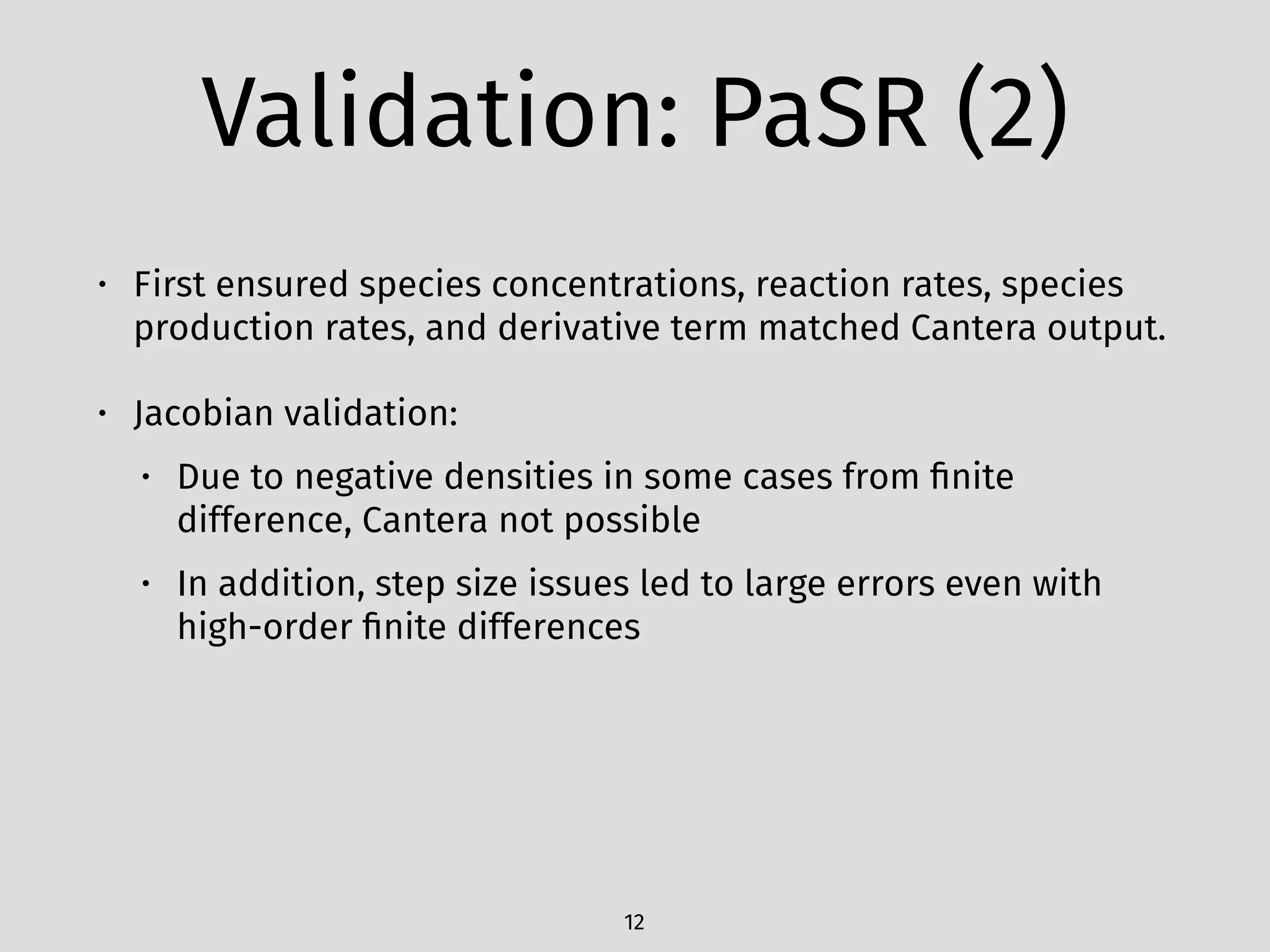
![Analytical Jacobian
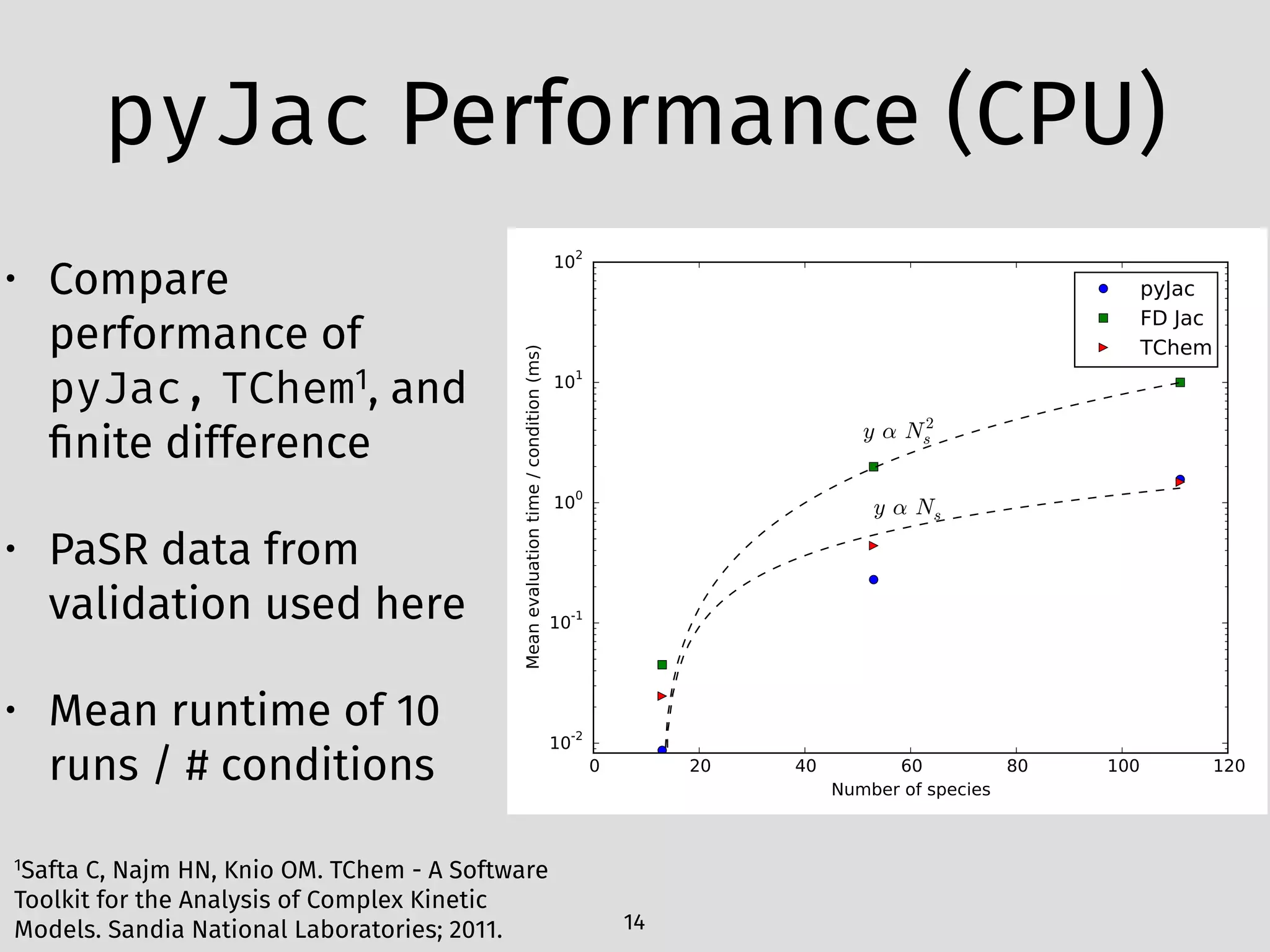
Following a lot of math…
8
Jk+1,1 =
Wk
⇢
✓
@ ˙!k
@T
+
˙!k
T
◆
=
Wk
⇢
NreacX
i=1
⌫ki
@ci
@T
(Rf,i Rr,i) + ci
✓
@Ri
@T
+
Rf,i Rr,i
T
◆
Jk+1,j+1 =
Wk
⇢
✓
@ ˙!k
@Yj
+ ˙!k
W
Wj
◆
=
Wk
⇢
"
˙!k
W
Wj
+
NreasX
i=1
⌫ki
✓
@ci
@Yj
(Rf,i Rr,i)
+ ci
Nsp
X
l=1
⌫0
li
W
Wj
Rf,i + ljkf,i
⇢
Wl
[Xl]⌫0
li 1
Nsp
Y
n=1
n6=l
[Xn]⌫0
ni
!
Nsp
X
l=1
⌫00
li
W
Wj
Rr,i + ljkr,i
⇢
Wl
[Xl]⌫00
li 1
Nsp
Y
n=1
n6=l
[Xn]⌫00
ni
!!!#](https://image.slidesharecdn.com/wsscif15pyjac-151005171629-lva1-app6892/75/Initial-investigation-of-pyJac-an-analytical-Jacobian-generator-for-chemical-kinetics-24-2048.jpg)
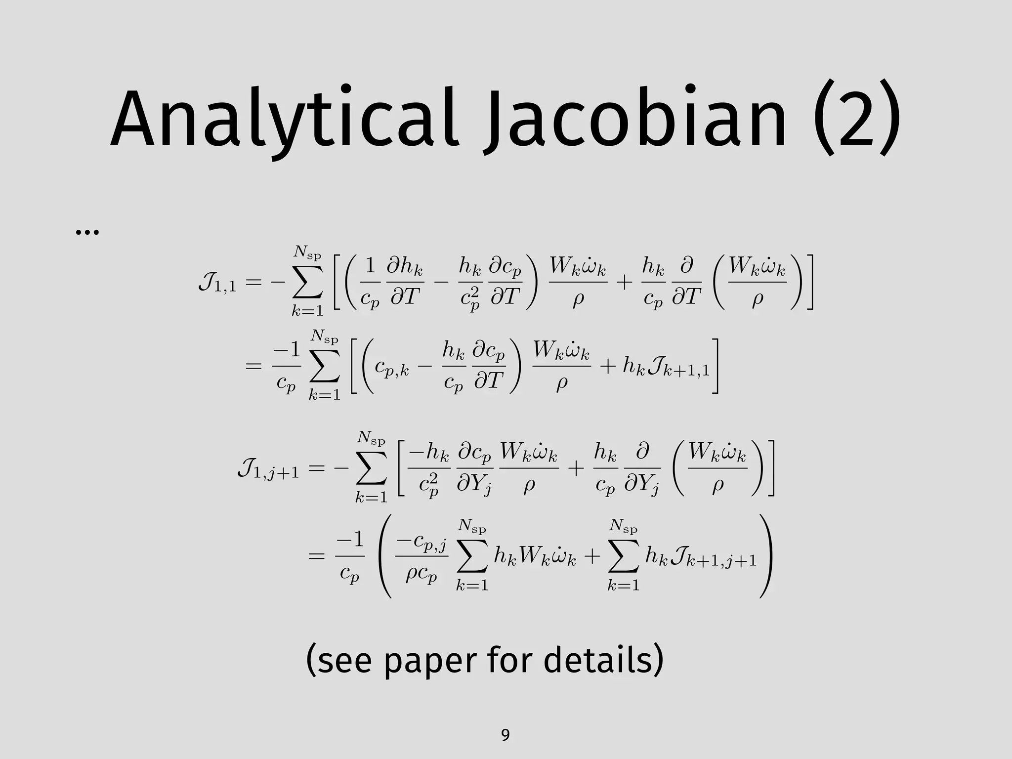


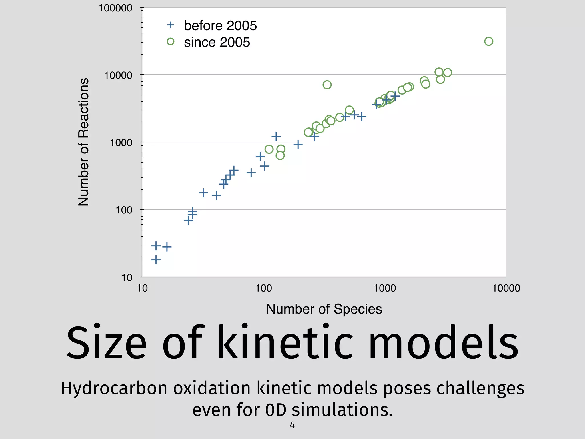
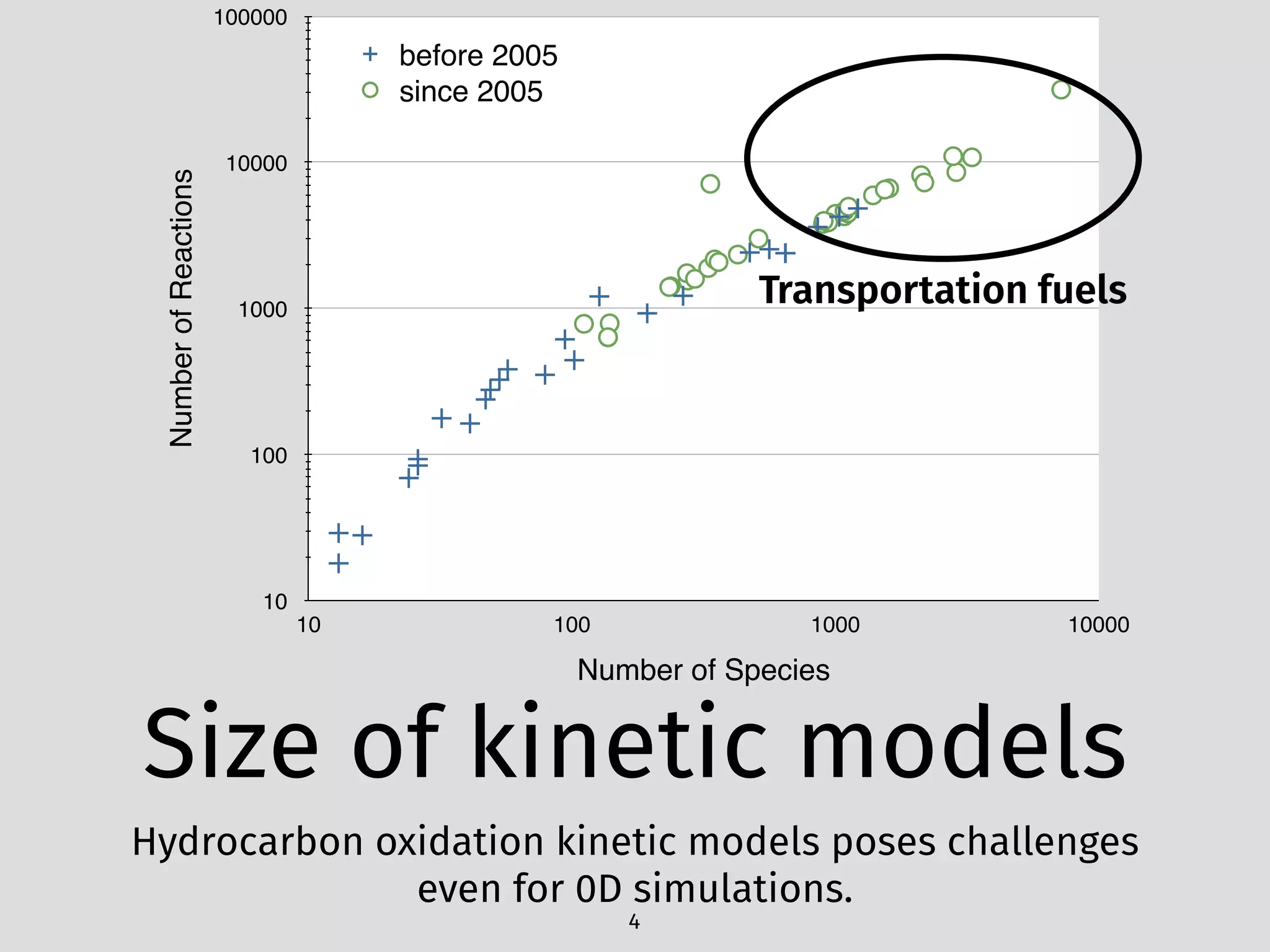
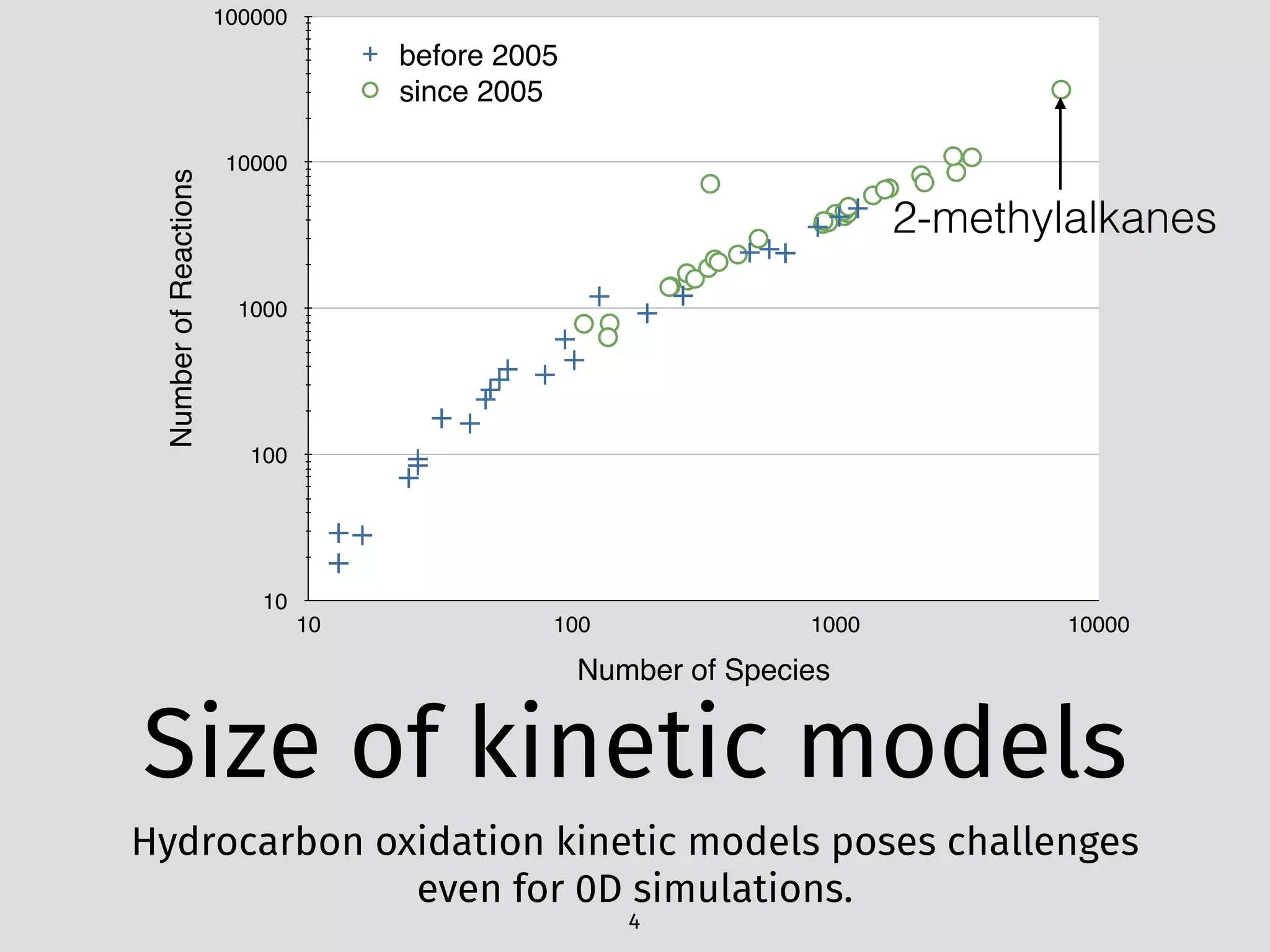
The document details an initial investigation of PyJac, an analytical Jacobian generator designed to streamline chemical kinetics integration, which is often hindered by stiffness in kinetic models. PyJac generates source code for both CPU and GPU architectures and is compatible with major chemical modeling platforms like Chemkin and Cantera. The validation results indicate that PyJac provides a significant improvement in computational efficiency over traditional methods in evaluating Jacobians for chemical reaction systems.


