Indexes overview

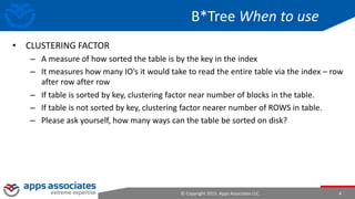
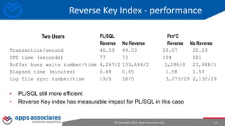
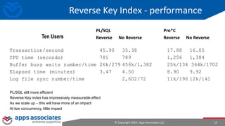
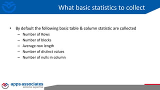
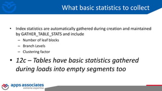
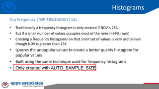
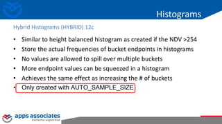
© Copyright 2015. Apps Associates LLC. 1
Performance Tuning Overview
March 30, 2015

Indexing

0..50
51..100
101..150
….
10000.. 10050
0..10
11..19
20..25
….
47.. 50
51..58
59..63
64..75
….
98.. 100
10000.. 10009
10010.. 10020
10021..10028
…
10046..10050
0,rowid
0,rowid
1,rowid
….
10,rowid
11,rowid
11,rowid
12,rowid
….
19,rowid
10046,rowid
10048,rowid
10048,rowid
….
10050,rowid
….
….
10021,rowid
10022,rowid
10023,rowid
….
10028,rowid
….
Create index I on T(numColumn)

B*Tree When to use
• CLUSTERING FACTOR
– A measure of how sorted the table is by the key in the index
– It measures how many IO’s it would take to read the entire table via the index – row
after row after row
– If table is sorted by key, clustering factor near number of blocks in the table.
– If table is not sorted by key, clustering factor nearer number of ROWS in table.
– Please ask yourself, how many ways can the table be sorted on disk?

1,Alice
2,Bob
3,Candy
4,Doug
5,Ellen
6,Frank
7,George
8,Hank
….
….
….
….
….
… …
…
…
…
….
0..50
51..100
101..150
….
10000.. 100500..10
11..19
20..25
….
47.. 50
51..58
59..63
64..75
….
98.. 100
10000.. 10009
10010.. 10020
10021..10028
…
10046..10050
….
Create index nm_idx on name)
Select * from t where pk between 1 and 8
Pk Name
1 Alice
2 Sue
3 Victor
4 Will
Pk Name
5 Irene
6 Kelly
7 Melanie
8 Oliver
Pk Name
9 George
10 Candy
11 Uwe
12 Wally
Pk Name
13 Ellen
14 Tom
15 Rick
16 Paul
Pk Name
17 Doug
18 Irene
19 Lance
20 Jack
Pk Name
21 Hank
22 Frank
23 Nicole
24 Bob

1,Alice
2,Bob
3,Candy
4,Doug
5,Ellen
6,Frank
7,George
8,Hank
….
….
….
….
….
… …
…
…
…
….
0..50
51..100
101..150
….
10000.. 100500..10
11..19
20..25
….
47.. 50
51..58
59..63
64..75
….
98.. 100
10000.. 10009
10010.. 10020
10021..10028
…
10046..10050
….
Create index nm_idx on name)
Select * from t where Name between ‘Alice’ and ‘Hank’
Pk Name
1 Alice
2 Sue
3 Victor
4 Will
Pk Name
5 Irene
6 Kelly
7 Melanie
8 Oliver
Pk Name
9 George
10 Candy
11 Uwe
12 Wally
Pk Name
13 Ellen
14 Tom
15 Rick
16 Paul
Pk Name
17 Doug
18 Irene
19 Lance
20 Jack
Pk Name
21 Hank
22 Frank
23 Nicole
24 Bob

Access paths – Getting the data
Access Path Explanation
Full table scan Reads all rows from table & filters out those that do not meet the where clause predicates. Used when no
index, DOP set etc
Table access by Rowid Rowid specifies the datafile & data block containing the row and the location of the row in that block. Used if
rowid supplied by index or in where clause
Index unique scan Only one row will be returned. Used when stmt contains a UNIQUE or a PRIMARY KEY constraint that
guarantees that only a single row is accessed
Index range scan Accesses adjacent index entries returns ROWID values Used with equality on non-unique indexes or range
predicate on unique index (<.>, between etc)
Index skip scan Skips the leading edge of the index & uses the rest Advantageous if there are few distinct values in the leading
column and many distinct values in the non-leading column
Full index scan Processes all leaf blocks of an index, but only enough branch blocks to find 1st leaf block. Used when all
necessary columns are in index & order by clause matches index struct or if sort merge join is done
Fast full index scan Scans all blocks in index used to replace a FTS when all necessary columns are in the index. Using multi-block IO
& can going parallel
Index joins Hash join of several indexes that together contain all the table columns that are referenced in the query. Wont
eliminate a sort operation
Bitmap indexes uses a bitmap for key values and a mapping function that converts each bit position to a rowid. Can efficiently
merge indexes that correspond to several conditions in a WHERE clause

Reverse Key Index
• Physically stores the bytes of the keys in reverse order
• In general, typically prevents range scanning
– 5 is not stored next to 6 is not stored next to 7…
• Used to avoid “hot block syndrome”
• Can also be used to avoid having to re-organize a ‘sweeping’ index

Reverse Key Index - performance
• It can help with buffer busy waits
– On monotonically increasing values
– Eg: sequence populated fields
– Eg: date/timestamp fields
• Especially in a clustered environment, this can reduce latency
• At the cost of additional CPU
– Evident mostly in single user mode
– When you go multi-user, because you are not spinning on a buffer wait, you see
less overall CPU

• PL/SQL still more efficient
• Reverse Key index has measurable impact for PL/SQL
Single User PL/SQL Pro*C
Reverse No Reverse Reverse No Reverse
Transaction/second 38.24 43.45 17.35 19.08
CPU time (seconds) 25 22 33 31
Buffer busy waits number/time 0/0 0/0 0/0 0/0
Elapsed time (minutes) 0.42 0.37 0.92 0.83
Log file sync number/time 6/0 1,940/7 1,940/7

CPU time (seconds) 77 73 104 101
Buffer busy waits number/time 4,267/2 133,644/2 3,286/0 23,688/1
Log file sync number/time 19/0 18/0 3,273/29 2,132/29
PL/SQL Pro*C
• PL/SQL still more efficient
• Reverse Key index has measurable impact for PL/SQL in this case
Two Users

PL/SQL still more efficient
Reverse Key index has impressively measurable effect
As we scale up – this will have more of an impact
At low concurrency, little impact
Ten Users
PL/SQL Pro*C
CPU time (seconds) 781 789 1,256 1,384
Buffer busy waits number/time 26k/279 456k/1,382 25k/134 364k/1702
Log file sync number/time 2,602/72 11k/196 12k/141

What basic statistics to collect
• By default the following basic table & column statistic are collected
– Number of Rows
– Number of blocks
– Average row length
– Number of distinct values
– Number of nulls in column

• Index statistics are automatically gathered during creation and maintained
by GATHER_TABLE_STATS and include
– Number of leaf blocks
– Branch Levels
– Clustering factor
• 12c – Tables have basic statistics gathered
during loads into empty segments too

• Histograms tell Optimizer about the data distribution in a Column
• Creation controlled by METHOD_OPT parameter
• Default create histogram on any column that has been used in the WHERE
clause or GROUP BY of a statement AND has a data skew
• Relies on column usage information gathered at compilation time and
stored in SYS.COL_USAGE$
Histograms

• 11g and before - Two types of histograms
– Frequency
– Height-balanced
• 12c and after – two more
– Top Frequency
– Hybrid
Histograms

Histograms
• A frequency histogram is only created if the number of distinct values in a
column (NDV) is less than 254 values
Frequency histograms (FREQUENCY)
Frequency histogram

Histograms
• A height balanced histogram is created if the number of distinct values in a
column (NDV) is greater than 254 values
Height balanced histograms (HEIGHT BALANCED)
Height balanced histogram

Histograms
• Traditionally a frequency histogram is only created if NDV < 254
• But if a small number of values occupies most of the rows (>99% rows)
• Creating a frequency histograms on that small set of values is very useful even
though NDV is greater than 254
• Ignores the unpopular values to create a better quality histogram for
popular values
• Built using the same technique used for frequency histograms
• Only created with AUTO_SAMPLE_SIZE
Top Frequency (TOP-FREQUENCY) 12c

Histograms
• Similar to height balanced histogram as created if the NDV >254
• Store the actual frequencies of bucket endpoints in histograms
• No values are allowed to spill over multiple buckets
• More endpoint values can be squeezed in a histogram
• Achieves the same effect as increasing the # of buckets
• Only created with AUTO_SAMPLE_SIZE
Hybrid Histograms (HYBRID) 12c

Indexes overview

Recommended

Recommended

More Related Content

What's hot

What's hot (20)

Viewers also liked

Viewers also liked (7)

Similar to Indexes overview

Similar to Indexes overview (20)

More from aioughydchapter

More from aioughydchapter (7)

Recently uploaded

Recently uploaded (20)

Indexes overview