This document discusses improving risk analysis in asset management by classifying failures according to their occurrence time. The current risk assessment may underestimate risks if failure probability and consequences are positively correlated. The document presents a case study analyzing transformer failure data from 2004-2010 based on occurrence time and associated load levels. Risk is reassessed using this improved classification approach. The results indicate risks may be underestimated by 7-13% without considering failure occurrence time.

1. J-7 2012 IEEE International Conference on Condition Monitoring and Diagnosis
23-27 September 2012, Bali, Indonesia
Improved Risk Analysis Through Failure Mode
Classification According to Occurrence Time
Ravish P.Y. Mehairjan, Qikai Zhuang, Dhiradj Djairam, Johan J. Smit
High Voltage Technology & Asset Management
Delft University of Technology
Delft, the Netherlands
r.p.y.mehairjan@tudelft.nl/ ravish.mehairjan@stedin.net
Abstract—Nowadays, risk-based asset management is outages, as the DNO is the only party who could prevent the
commonly adopted throughout electricity utilities as a business outage or limit their consequences [2]. However, the end-
model. Potential risks are registered, and after selection the user of electricity can generally not be expected to be
influence of the risk is assessed. This paper discusses the interested in the cause of an outage, as it is the end-result
possible shortcomings with regard to current risk assessment rather than the cause that would interest him. Literature
methods. Based on an improved risk assessment approach, it is shows [3] that the end-user is also interested in the timing of
shown that risk might be underestimated when the economic an outage i.e. the time at which the outage occurred. This has
loss of failures are not incorporated in the assessment. a direct impact on the costs.
Furthermore, with the advent of the intelligent networks of the
Different customers (groups) value outages differently.
future (intelligent grid), the more user-centric requirements
Interruption costs are driven by a number of factors and has
should anticipate an improved risk assessment approach for
asset management. Moreover, emerging dynamic pricing, been extensively studied in literature [3]. Amongst others,
demand-side-management, two-way information transfer, etc., one of the influencing factors is the timing, or rather
might provide tools to measure the reliability indicator occurrence time, of outages. Interruption costs varies in
“Energy Not Supplied” even at distribution network levels. In accordance to the time in the year, day in the week and time
this contribution, a case study of 50/10 kV transformer failures in the day. This is also dependent on the type of customer.
is analysed according to the failure occurrence time and loss of For example, for residential customers, winter interruptions
load. The results are applied as input for an improved risk have higher impact than summer interruptions. Likewise,
assessment approach, which, ultimately, reveals that risks are morning or afternoon interruptions are less costly than
likely to be underestimated. In conclusion, we show that evening ones [3]. Yet, many European regulators have
without considering the occurrence time of failure, the risks of agreed to regulate DNOs on their average performance
failures will be underestimated for 7% to 13%. namely, SAIFI and SAIDI [4]. The disadvantage of
averaging is that detailed information is lost e.g. when all
Keywords- risk; failure occurrence time; asset management. failures are in the peak hours of the load, the amount of
interrupted customer is the same when compared to the off-
I. INTRODUCTION
peak hours, however the economic value of the failures in
Generally, the main objectives of power sector reform is to peak hours is significantly higher. A potential method to
improve quality and efficiency levels [1]. Regulators are avert this shortcoming might be to apply the “Energy Not
responsible for monitoring quality of supply and, Supplied (ENS)” rather than SAIDI/SAIFI as is done for
additionally, promote high economic efficiency. To most example in Norway [5].
customers, network reliability is important with regard to Usually, ENS is measured on transmission system level and,
quality of supply. Therefore, network reliability is prioritised because of lack of measurements, it has not been extensively
by regulators when starting regulating quality of supply. For applied on distribution system level [2]. Meanwhile, the
Distribution Network Operators (DNOs), the most transition towards intelligent grids imposes significant
commonly used indicator for network reliability by European challenges on network companies. While there is no single
regulators are [1]: definition for intelligent grids, there is consensus that such a
- SAIDI (System Average Interruption Durations grid will be; user centric, and focused on outputs [3]. It is
Index, which provides a measure of average time also accepted that the challenges will be different for
that customers are interrupted) transmission and distribution with the potential planning and
operational changes being more significant for distribution
- SAIFI (System Average Interruption Frequency networks. One of the main priorities for regulators is to focus
Index, which measures the number of outages more on the output of network operators [6].
experienced by customers) With the advent of the intelligent grid and its capabilities, the
asset manager will be expected to reconsider the way risks
Additional to legal obligations of the regulator, most DNOs
are assessed. This paper argues that the dynamic energy price
employ detailed key performance indicators (KPI’s) such as,
(changing energy price according to demand, also known as
causes of interruptions, worst served customer, etc.
demand-side management) in the scenario of an intelligent
Regulators consider the DNO to be the responsible party for
This research has been performed in close collaboration with Stedin (a
Dutch Distribution Network Operator, DNO) and reviewed by Dr. Viren
Ajodhia (DNV KEMA).
978-1-4673-1018-5/12/$31.00 ©2012 IEEE
866

2. grid potentially creates hazards in the risk assessment overestimated when F and C are positively correlated and
process. In section II, we discuss that expected failure loss underestimated when they are negatively correlated. In the
can be underestimated when the failure probability and current situation, the uncertainty of C is mainly caused by
consequences are positively correlated. This is typical when mixing failure modes, i.e. failures of different causes and/or
both demand and price for electricity increase in different components are analyses as follows; their time-
simultaneously. In section III, an approach to address this to-failure are fitted into a single probability distribution such
problem is proposed. Here, failures are investigated, not only as figure 1. Consequently, F and C are negatively
according to their technical cause, but also their occurrence correlated, because failures with larger impacts and/or
time.
components with higher ratings tend to occur less
II. ASSET MANAGEMENT frequently. This leads to an overestimation of the risk,
which is preferred by the asset manager rather than the
A. Current Risk Assessment Approach opposite. However, in a future intelligent grid scenario with
Asset management (AM) is a discipline with growing e.g. dynamic energy pricing, it is expected that a positive
importance in European utility companies [7]. In a utility correlation between failure probability and consequence will
company, the asset manager connects the asset owner, who occur. For example, in a high demand period, the price of
operates and invests on the network, with the service energy will increase. As a result of the high demand (load),
provider, who maintains and monitors the components [7]. the temperature of assets is expected to increase, which
The goal of AM is to optimize the cost, performance and ultimately accelerates aging and increases failure probability
risks of the assets through proper decision making processes of power system components, such as cables, transformers,
[7]. In today’s AM, the process of “risk register” is overhead lines, etc. Thus, one could argue that time
commonly applied to understand the effect of failures on the intervals of higher prices tend to be linked with increased
company and the society. Typically, a category of failures is possibility of failures. Hence, a potential underestimation of
registered as a risk with information about the probability risks according to current risk assessment methods.
and consequences. Risks are compared to each other Therefore, the asset manager might need to apply
according to their expected loss, namely the product of modifications in the risk assessment.
multiplying probability (e.g. in figure 1) with consequence.
C. Research Approach
The risk, is assessed through equation (1):
In this contribution, a possible solution to deal with the
. 1 preceding problem about risk assessment in the future is
discussed. A case study with transformers at distribution
where E() is the expected value, R is the economic output of level regarding their failure data and load profile data is
the risk, F is the failure probability and C is the failure analysed. In figure 2, the steps followed in this study are
consequence. Risk assessment can be accomplished through shown. The improved risk analysis is incorporated, shown
applying risk matrix [9]. in the orange boxes. The failure data for 50/10 kV
transformers are divided into multiple groups according to
the occurrence time of the failures. Similar to the grouping
of the failures, the historic load data for the transformers is
classified for the same occurrence time intervals.
Failure
Data Correlation
Failure
Probability
Failure Estimation
Time
Risk
Figure 1: Example of fitting time-to-failure data into a Weibull distribution Assessment
(in left figure) and estimating failure rate vs. service age (right figure) of
distribution transformer [8]. The predicted failure rate can be further used
in the “Probability” column of Table 1. Transformer Failure
load Consequence
Figure 2: Research approach applied in this paper. The black boxes and
B. Problem Statement
arrows indicate the current Risk Assessment procedure. The orange boxes
The implementation of equation (1) is straightforward and arrows indicate the improved Risk Assessment.
because of a practical reason: the occurrences of failures can
be predicted scientifically by asset workers and service III. IMPROVED RISK ASSESSMENT
providers with technical backgrounds while the failure costs A. Failure Data Analysis
are predicted economically by stakeholder relationship As mentioned previously, failure data of 50/10 kV
departments of asset owners. Equation (1) is correct only transformers are analysed. Failure data for the period 2004-
when C is deterministic, or when C is a random variable 2010 was consistently available from a Dutch DNO. Instead
independent from F. In other words, the risk will be
867

3. of calculating the failure rates based on the physical cause
e week, the average load for the particular time interval has
of the failure, a correlation between th failure data
he been estimated. Two types of transformer loading have been
according to the occurrence time (time of in nterruption) was considered, namely: industri + residential (region 1) and
ial
considered. The authors prefer to estimate a failure rate
e residential + commercial (reegion 2). The load classification
invariant with the service age, because of tw facts: Firstly,
wo according to specific time in
ntervals for summer and winter
the failure data is available for only 7 years This period is
s. loads for region 1 and 2 are given in table 3 and 4,
insufficient to reflect the aging phase of transformer respectively.
lifecycle which is typically several decades Secondly, the
s.
concern of this paper is to indicate the corr relation between
failures and their occurrence time. Therefore the application
e,
of life data analysis, such as fitting time-to-failure data into
a Weibull distribution is not necessary, s since its output
mainly reveals the aging of asset population at a yearly time
frame.
The service-age-constant failure rate can b calculated as
be
follows. Firstly, since failures before 2 2004 were not
recorded, the operation time of the who transformer
ole
population is neglected. 86 transformers hav been operated
ve
between 2004 and 2010, and 2 new tran nsformers were
installed in 2009. Accordingly, the total tr ransformer year
number, label as n in the below equations, is 86*7+2=806. Figure 3: Week (11 June 2012 – 18 June 2012) load profile for 2
transformers in a substation of regio 1.
on
Naturally, the failure rate can be estimated as k/806, where k
s
is the total number of recorded failures with specified Summer Load
S Winter Load
occurrence time, in our case. Secondly, s since the failure Region 1 Failure TR1
T TR2 TR1 TR2
rate is constant, the total number of fail lures follows a Occurrence Load
L Load Load Load
binominal distribution. Since n is large, the binominal Industrial Time Interval (M
MW) (MW) (MW) (MW)
distribution is approximately a Poisso distribution.
on + 0:00 - 06:00 4.87 4.72 5.12 5.68
Residential 06:00 - 12:00 9.39 9.37 10.70 10.75
Therefore, the 90% confidence interval of the failure rate
12:00 - 18:00 10.21 12.65 13.69 11.78
estimation can be calculated through the χ2 p percentiles in the 18:00 - 24:00 7.73 8.27 9.52 9.77
two equations below. Total 32.20 35.01 39.03 37.98
, % Table 3: Summary of analysed ave erage transformer load data categorized
according to time intervals for reg gion 1 with industrial and residential
2 loads. In this substation 2 transform are used and arbitrarily named TR1
mers
, % and TR2.
2
2
From the above steps, the failure rates can be estimated with
e Summer Load Winter Load
Region 2 Failure TR1 TR2 TR1 TR2
confidence intervals as below: Occurrence Load
L Load Load Load
Commercial Time Interval (MW)
( (MW) (MW) (MW)
Failure # of Upper Failuure Lower + 0:00 - 06:00 4.04 4.37 3.80 4.48
Occurrence failures Conf. Ratte Conf. Residential 06:00 - 12:00 5.80 6.09 6.28 8.22
Time Interval Bound Bound 12:00 - 18:00 6.84 7.07 7.26 9.92
0:00 - 06:00 1 0,0079 0,0017 0,0001 18:00 - 24:00 5.40 5.74 6.19 8.53
06:00 - 12:00 8 0,0239 0,01333 0,0066 Total 22.08 23.27 23.53 31.15
12:00 - 18:00 7 0,0218 0,0116 0,0055 Table 4: Summary of analysed ave erage transformer load data categorized
18:00 - 24:00 7 0,0218 0,0116 0,0055 according to time intervals for reg gion 2 with commercial and residential
Total 23 0,054 0,03881 0,0261 loads. In this substation 2 transform are used and arbitrarily named TR1
mers
Table 2: 50/10 kV transformer failure data categorized according to failure and TR2.
occurrence time intervals.
C. Risk Assessment
B. Transformer Load Data
As mentioned earlier, equat tion (1) is used in the current
As mentioned previously, interruption cos hence sales
sts, situation to assess the risks. For the proposed improved risk
loss and interruption costs, varies according to the time of
g assessment, equation (1) is extended with more detailed
s
the interruption. To take this into account tr ransformer load information regarding the f failure occurrence time, and is
data for a period of 1 week for a summer an winter season
nd mathematically expressed as follows:
are analysed. A summer load for a period of 1 week is
d
shown in figure 3. Similar to the time inter rvals as defined . .
for the failure rates, the transformer load data is categorized.
a
Notably, no correlation between recovery duration and
y ... . ... . 3
failure occurrence time has been found. Over the period of 1
r
868

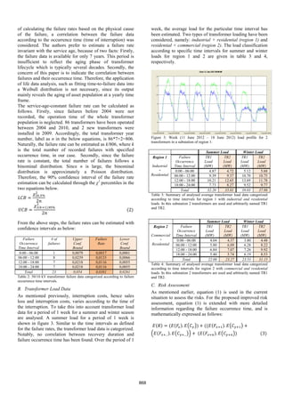
4. with, Fx being the failure probability for a particular time and failure modes. Therefore, we strongly recommend
interval and Cy the loss of load for the same time interval. utility companies to reconsider their information strategies,
Subsequently, equations (1) and (3) are used to assess the or at least investigate on possible factors which leads to
under- or over estimation of risk when the failure correlation between failure rates and consequences.
occurrence time is considered.
IV. CONCLUSION
Current Risk Improved Risk Improved/Current This study analyse risk of transformer failures with a
Region 1 TR1 TR2 TR1 TR2 TR1 TR2 differently defined failure consequences. The consequences
are assumed to be proportional to the load of the
Summer 0.31 0.33 0.34 0.37 11% 13%
Winter 0.37 0.36 0.42 0.40 13% 11%
transformer, which leads to a correlation between failure
Table 5: Improved risk assessment results. When load (loss of energy) is consequences and occurrence time. Meanwhile, the
incorporated, according to failure occurrence time, then there is an estimated failure rate also shows the same correlation with
estimated risk underestimation between 11% - 13% for region 1. occurrence time. As a result, we have shown that: without
considering the occurrence time of failure, the risks will be
Current Risk Improved Risk Improved/Current underestimated for 7% to 13%, depending on the above-
Region 2 TR1 TR2 TR1 TR2 TR1 TR2
stated correlations which is associated with other factors
Summer 0.21 0.22 0.23 0.24 7% 7% (e.g. season, type of feeding area).
Winter 0.22 0.29 0.25 0.33 10% 11% To expand this simplified analysis, we recommend to (1)
Table 6: Improved risk assessment results. When load (loss of energy) is find out the reasons for the statistically estimated correlation
incorporated, according to failure occurrence time, then there is an between failure rate and time; (2) investigate on the repair
estimated risk underestimation 7% - 11% for region 2.
duration, so that the lost energy instead of load can be used
for the failure consequences; (3) in long term, investigate on
From tables 5 and 6, it is found that with the current risk
the demand-side and understand the impact of failures on
assessment approach an underestimation of risks is likely to
clients.
occur. When the “current” risk analysis method is compared
To sum up, it is still unclear, whether utilities are aware of
to the “improved” risk analysis, then there is a possible risk
these shortcoming in current risk assessment methods and
underestimation between 7% - 13%. Furthermore, we can
how to incorporate these results into AM in practise.
conclude from this primary investigation that for the winter
Besides, it also remains unclear what the consequences of
load period the risk uncertainty is slightly larger (about 3%
these results are for utilities in terms of maintenance and
to 4%) when compared to the summer load period.
operations. In future, with the roll-out of intelligent grids
Additionally, we can tentatively conclude that region 1,
and increased user-centric involvement, improved risk
which has a dominant industrial load, has a higher risk
assessments may become a serious topic of discussion.
uncertainty exposure. These seasonal and regional
difference are caused by the fact that the underestimation ACKNOWLEDGEMENT
grows with the ratio between peak load and basic load.
The authors would like to thank Stedin B.V. and Dr.
D. Discussion Viren Ajodhia (DNV KEMA) for their support, knowledge
Here, the load is assumed proportional to the failure and access to data.
consequence, hence used to calculated risk directly. Based REFERENCE
on this assumption, the results show a case that failure
[1] V.S. Ajodhia, “Regulation beyond price: integrated price-quality
interruption costs can include any component of cost that regulation for electricty distribution networks”, Ph.D Dissertation,
are associated with asset failure, therefore, the calculated Delft University of Technology, the Netherlands, 2006.
risk differences might even be more serious to the asset [2] K. Keller, B.F.C. Franken, “Quality of Supply and Market
managers. Regulation: survey within Europe”, KEMA Consulting, 2006.
The authors realize that, in practise, failure costs can related [3] D. Caves, J. Herriges, R. Windle, “Customer Demand for Service
Reliability in the Electric Power Industry: A Synthesis of the Outage
to many other factors, such as additional emergency service Cost Literature”, Bulletin of Economic Research, 2:79-119, 1990.
costs, the cost of degraded operations, environmental costs, [4] CEER, “5th CEER Benchmarking Report on the Quality of Electricty
and loss of customer goodwill. These factors, in case that Supply 2011”, 2012.
they are correlated with time, season and region, can further [5] F. Trengereid, "Quality of supply regulation in Norway", Norwegian
increase the underestimation of risk values. water resources and energy directorate (NVE), 2003.
These cost factors are not taken into account in the current [6] European Regulators Group for Electricity and Gas EREG, “Posistion
study, because relevant data are not recorded. This reveals a Paper on Smart Grids”, ERGEG, 2010.
shortcoming of failure analysis in the utility companies at [7] The Institute of Asset Management (IAM), “Asset Management- an
anatomy”, Issue 1, dec 2011.
this moment: The organization within utility companies
[8] L. Chmura, P.H.F. Morshuis, E. Gulski, A. Janssen, “Statistical
separate the investigations on failure probability and those analysis of subcomponent failures in power transformers”, EIC –
on failure consequences within technical and financial Electrical Insulation Conference, Annapolis, Maryland, USA, 2011.
department respectively. Consequently, failure analysers can [9] Cigre WG C1.1, “Asset Management of Transmission Systems and
hardly trace the association between failure consequences associated cigre activities”, Cigre Techical Brochure 309, 2006.
869