SlideShare a Scribd company logo
Immigration and Reviatilzation in Philadelphia
Jake Riley
Overview
The goal of my project is to look at demographic shifts in the foreign-born community in Philadelphia between 1970-
2010. It can easily be argued that Philadelphia (and many urban areas) has been actively devitalized since the 1970s. As
will be shown in this project, Philadelphia lost over 300,000 residents in the 1970s, a reduction of over 13%. This is
equivalent to half of the residents in Washington, DC leaving Philadelphia in the span of 10 years. In each subsequent
census, the trend continued until a slight increase occured in 2010. Closer analysis of this 1% population increase shows
that the growth is attributed to an increase in foreign-born residents in Philadelphia. This project seeks to explore the
changing demographics within the city.
Introduction
In this project I will explore the research question "What is the relationship between immigration and revitalization in
Philadelphia?". I started this project last semester in a studio class and want to replicate the results in R. In my previous
project, I attempted to match 1980 census data to 2010 and was unable to analyze tracts that had changed boundaries. In
revisiting this research question, I was able to locate data sources that allow me to conduct a longitudinal analysis via
crosswalk tables from National Historic GIS (NHGIS) and the Longitudinal Tract Database (LTDB). The story regarding
"urban revitalizaion" is often discussed through the process of gentrification. Using the knowledge that I gained from
previous work on this subject, I will show that Philadelphia's population growth, as well as elements associated with
revitalization, is heavily impacted by demographic shifts in the native and foreign born communities within the city-
limits.
This problem is interdiciplinary because it spans several fields. Through coding in R, there is a heavy data science
component, there are also insights gained from geography, criminology, sociology, and demography. I will start with an
overview of the city's native- and foreign-born populations. I will then break out each group into more specific "place of
birth" categories to understand migratory patterns within the United States for the native-born, and country of origin for
the foreign-born. I will also look at the changes in these demographics over time by examining census data between 1980
and 2010. I had originally hoped to explore the relationship of the foreign-born population to areas considered key
factors in revitalization: commercial activity and safety. However, I decided to make the code dynamic so that it is able to
look at any county in the nation. It is my hope to turn this into a shiny app and have it be available to the public. I have run
this file twice, once for Philadelphia and once for Washington, DC. I will compare the results of Philly as it relates to DC.
This version has the code; the other two files are just the graphs and charts.
It is my hope that the results of this project act as a catalyst for future research. The dominant narrative regarding
revitalization generally lacks a nuanced discussion on immigration. My belief is that this portfolio will add complexity to
the way we describe the growth of urban areas. It is also my hope that immigrant communities will be acknowledged for
their contributions in Philadelphia and that government officials will build policies that consciously support the foreign-
born residents who are here, and those yet to come.
Methods
I will utilize data from the National Historic GIS NHGIS, the Longitudinal Tract Database LTDB, and data related to land
use and crime through OpenDataPhilly. NHGIS has allowed the census to be studied longitudinally by standardizing
questions over time. The wording of both questions and answers have changed over time and so NHGIS has identified the
variable names for questions that are consistently asked and arranged them into time-series data sets. In particular, I will
be looking at questions regarding count of persons by nativity (native-born vs foreign born), native-born persons by place
of birth, and foreign-born persons by place of birth. In a similar manner, the LTDB creates crosswalk tables to compare
changes in geography over time. Because census tract boundaries change as populations grow and decline, the LTDB has
calculated the approximate area of a tract in 2010 that was formerly part of a census tract (or tracts) in previous decades.
Doing so allows social scientists to compare geographic areas using a singular data set (in this case the 2010 census
boundaries) and identify demographic shifts by census tract. I will combine the NHGIS data with the LTDB data and
invesitigate several relationships between the native- and foreign-born communities.
R Code:
library(RCurl)
library(tidyr)
library(dplyr)
library(ggplot2)
library(ggmap)
library(foreign)
library(rgdal)
library(rgeos)
library(maptools)
library(RColorBrewer)
library(stringr)
library(shapefiles)
library(knitr)
options(scipen=999)
#These two variables identify the FIPS code for the state and county of interest. These are the only two variables that n
eed to be changed to create different county profiles.
#State should be 2 characters with leading zero
stateFIPS <- '42'
#NHGIS has county as numeric
countyFIPS <- 101
#Examples State County
#Philadelphia 42 101
#DelCo PA 42 45
#DC 11 1
#MontCo MD 24 31
#Baltimore 24 510
#Atlanta 13 121
#Portland 41 51
#San Francisco 06 75
#These two variables will be used to filter data later in the script
findFIPS <- paste(stateFIPS,str_pad(countyFIPS, 3, pad="0"),sep="")
filterFIPS <- paste("^",findFIPS,sep="")
#Bring in codebook to give readable titles to variable names
Codes <- getURL("https://raw.githubusercontent.com/rjake/FinalProject/master/Codebook.csv")%>%read.csv(text=., header = T
RUE, sep=",", stringsAsFactors = FALSE)%>%as.data.frame()
#Codes <- read.csv("Codebook.csv",stringsAsFactors=FALSE)%>%as.data.frame()
#read in county level NHIS data
County <- getURL("https://raw.githubusercontent.com/rjake/FinalProject/master/nhgis_ts_nominal_county.csv")%>%read.csv(te
xt=., header = TRUE, sep=",",stringsAsFactors=FALSE,na.strings=c("", "NA"))%>%as.data.frame()
#County <- read.csv("nhgis_ts_nominal_county.csv",stringsAsFactors=FALSE,na.strings=c("", "NA"))%>%as.data.frame()
#CityName will be used in the titles of charts and tables and to filter data later in the script
CityName <- ifelse(stateFIPS=="11", paste("District of Columbia"),
filter(County,(STATEA==stateFIPS) & (COUNTYA==countyFIPS)& (YEAR=="2008-2012"))%>%
select(COUNTY,STATE)%>%
slice(1)%>%
paste(collapse=", "))
City <- County %>%
filter((STATEA==stateFIPS) & (COUNTYA==countyFIPS)) %>%
select(-ends_with("M")) %>%
select(which(unlist(lapply(., function(x)!all(is.na(x))))))%>% #Removes any black columns
select(-c(1,3:7)) %>%
gather("Var","Total",-1) %>%
left_join(filter(Codes,File=="NHGIS"), by="Var")
Results
First I will show the changes across the county from 1970-2010
#Net Population Growth
TotalPop <- City%>%
filter(Question == 'Citizenship')
TotalPop$Pop <- TotalPop$Pop %>%
as.factor()%>%
factor(., levels=rev(levels(.)))
#As stacked bar chart
ggplot(TotalPop, aes(YEAR,Total, fill=factor(Pop), order=Pop))+
geom_bar(stat="identity", color="black")+
scale_fill_manual(values=c("gray40", "gray70"))+
theme_bw()+
ggtitle(paste("Population Totals for Native & nForeign Born Residents","nfor ",CityName,sep=""))+
theme(plot.title = element_text(hjust = 0,size=12))
#Table showing difference in total population between decades
TotalPop%>%
group_by(YEAR)%>%
summarise(Total=sum(Total))%>%
as.data.frame()%>%
mutate(Diff=lead(Total)-Total)%>%
mutate(Change=paste(round(Diff/Total ,3)*100,"%", sep=""))%>%
kable()
YEAR Total Diff Change
1970 1948608 -260398 -13.4%
1980 1688210 -102633 -6.1%
1990 1585577 -68027 -4.3%
2000 1517550 8261 0.5%
2008-2012 1525811 NA NA%
#As a line graph
ggplot(TotalPop, aes(YEAR,Total,Pop,group=Pop,color=Pop))+
geom_line(size=1,linetype = 2)+
geom_point(size=4.5)+
scale_color_manual(values=c("black", "gray40"))+
theme_bw()+
ggtitle(paste("Population Totals for Native & nForeign Born Residents", "nfor ",CityName,sep=""))+
theme(plot.title = element_text(hjust = 0,size=12))
Analysis Similar to DC, Philadelphia took a hit in the 1970s. Philadelphia dropped 13.4% between 1970 and 1980 (~260,400 people)
while DC dropped 15.6% (~118,200 people). Both cities continued to decrease in population until the 2010 census where DC saw a large
increase of 5.9% (~33,700 people). Philadelphia grew as well, but much less so (<1%, ~8,000 people). The graphs for Philadelphia show
that, although there was an increase, the increase is due to the increasing size of the foreign-born population; the native-born population,
as a whole, continues to decline.
Here I break out the proportion of native born residents who are born in state vs. those born in another state.
#Native Born
NBorn <- City %>%
filter(Pop=="Native Born" & Question=="Place of Birth")%>%
filter(Qual=='In State'|(Qual=='Other State' & Qual2=='total'))
#total pop
ggplot(NBorn, aes(YEAR,Total, fill=factor(Qual), order=Qual))+
geom_bar(stat="identity")+
scale_fill_manual(values=c("gray40", "gray70"))+
theme_bw()+
ggtitle(paste("Native Born Residents in n",CityName,sep=""))+
theme(plot.title = element_text(hjust = 0,size=12))
#born in state or in another state
ggplot(NBorn, aes(YEAR,Total,Qual,group=Qual,color=Qual))+
geom_line(size=1,linetype = 2)+
geom_point(size=4.5)+
scale_color_manual(values=c("black", "gray40"),name = "Place of Birth")+
theme_bw()+
ggtitle(paste("Native Born Residents in n",CityName,sep=""))+
theme(plot.title = element_text(hjust = 0,size=12))
Analysis Philadelphia's In state residents make up tha majority of the native-born population in Philadelphia. The born-in-state
residents have declined at a steady rate each decade and those born out of state appear to be growing, though slowly. In DC, a different
ratio exists. In the nation's capitol, more than half of the residents are born out of state and this trend has existed in each of the observed
decades.
Here I look at each region separately
#by specific location
NBorn2 <- City %>%
filter(Pop=="Native Born" & Question=="Place of Birth")%>%
filter(Qual=="Other State" & Qual2!="total")
#each year by Region
ggplot(NBorn2, aes(YEAR,Total))+
geom_bar(stat="identity")+
facet_wrap(~Qual2, ncol=4)+
theme_bw()+
ggtitle(paste("Birth Place of Native Born Residents in n",CityName," by Region",sep=""))+
theme(plot.title = element_text(hjust = 0,size=12))+
theme(axis.text.x = element_text(angle = 90, hjust = 1))
#each region by year
ggplot(NBorn2, aes(Qual2,Total))+
geom_bar(stat="identity")+
facet_wrap(~YEAR, ncol=5)+
theme_bw()+
ggtitle(paste("Birth Place of Native Born Residents in n",CityName," by Year",sep=""))+
theme(plot.title = element_text(hjust = 0,size=12))+
theme(axis.text.x = element_text(angle = 90, hjust = 1))+
scale_x_discrete(name="")
Analysis The first chart (for Philadelphia) shows that migration from the South was most pronounced in the 1970s and 1980s and has
since lowered. The Northeast and West are increasing, with the Northeast becoming the largest group represented in Philadelphia. In DC,
the trend has been similar, but the South is still the largest group represented by those who live in DC and were born out-of-state.
Here I look at foreign-born residents:
#Foreign Born
#This is the main table used to create the other two tables, place of birth (Qual2) is more specific (Ex. N. Europe, Chin
a)
FBornSpec<-City %>%
filter(Pop=="Foreign Born" & Question=="Place of Birth") %>%
filter(YEAR!=1980 & YEAR!=2000)
#This is a more generalized location for place of birth (Ex. Europe, Asia)
FBornGen <- FBornSpec %>%
group_by(YEAR,Qual)%>%
summarise(Total=sum(Total))%>%
filter(!is.na(Total))
#This is the total Count for each decade
FBornTotal <- FBornGen %>%
group_by(YEAR)%>%
summarise(Total=sum(Total))%>%
mutate(Pop='Foreign Born')
#total foreign-born pop by year
ggplot()+
geom_bar(data=FBornGen, aes(YEAR,Total, fill=Qual),color="black", stat="identity", position="dodge")+
scale_fill_brewer(palette="PRGn")+
geom_point(data=FBornTotal, aes(YEAR, Total,Pop,group=Pop),size=3.5, color="grey40")+
geom_line(data=FBornTotal, aes(YEAR, Total,Pop,group=Pop),size=1, color="grey40", linetype=2)+
theme_bw()+
ggtitle(paste("Birth Place of Foreign Born Residents nand Total Foreign-Born Population", "nin ",CityName," by
Year",sep=""))+
theme(plot.title = element_text(hjust = 0,size=12))
#by location
ggplot(FBornGen, aes(YEAR,Total))+
geom_bar(stat="identity")+
facet_wrap(~Qual, ncol=6)+
theme_bw()+
ggtitle(paste("Population Totals for Foreign Born Residents in n",CityName," by Region ",sep=""))+
theme(plot.title = element_text(hjust = 0,size=12))+
theme(axis.text.x = element_text(angle = 90, hjust = 1))
Analysis From these two charts you can see that Europeans were the largest immigrant group in Phildelphia in the 1970s and have
signficiantly declined. Groups from Africa, the Americas (Central & South), and Asia have been growing each decade, and Asian
immigrants are currently the largest represented immigrant group in Philadelphia. DC shows a different trend. In DC, Europeans have
been relatively the same in number overtime while groups from Africa, Asia, and most dramatically, the Americas have grown in size
from one census to the next. (Note: this question was asked every other decade.)
To compare tract growth, I had to create crosswalk tables from the LTDB and NHGIS data.
#TRACT GROWTH
#Read in each crosswalk table, format correctly then rowbind
LTDBx1970 <-
getURL("https://raw.githubusercontent.com/rjake/FinalProject/master/LTDB%20crosswalk_1970_2010.csv")%>%read.csv(tex
t=., header = TRUE, sep=",",stringsAsFactors=FALSE,na.strings=c("", "NA"))%>%
# read.csv("LTDB crosswalk_1970_2010.csv",stringsAsFactors=FALSE)%>%
#add year of original tract column
mutate(YEAR=1970)%>%
#add leading zeros to FIPS, combine with year to create a look up to match with NHGIS census tract data (below)
mutate(tractid=str_pad(trtid70, 11, pad="0"))%>%
mutate(LOOKUP=paste(YEAR,tractid,sep="_"))%>%
#subset to City tracts
filter(substr(tractid,1,5)==findFIPS)%>%
#select uniform columns
select(YEAR, LOOKUP, weight, trtid10)
LTDBx1980 <-
getURL("https://raw.githubusercontent.com/rjake/FinalProject/master/LTDB%20crosswalk_1980_2010.csv")%>%read.csv(text=
., header = TRUE, sep=",",stringsAsFactors=FALSE,na.strings=c("", "NA"))%>%
#read.csv("LTDB crosswalk_1980_2010.csv",stringsAsFactors=FALSE)%>%
mutate(YEAR=1980)%>%
mutate(tractid=str_pad(trtid80, 11, pad="0"))%>%
mutate(LOOKUP=paste(YEAR,tractid,sep="_"))%>%
filter(substr(tractid,1,5)==findFIPS)%>%
select(YEAR, LOOKUP, weight, trtid10)
LTDBx1990 <-
getURL("https://raw.githubusercontent.com/rjake/FinalProject/master/LTDB%20crosswalk_1990_2010.csv")%>%read.csv(text=
., header = TRUE, sep=",",stringsAsFactors=FALSE,na.strings=c("", "NA"))%>%
#read.csv("LTDB crosswalk_1990_2010.csv",stringsAsFactors=FALSE)%>%
mutate(YEAR=1990)%>%
mutate(tractid=str_pad(trtid90, 11, pad="0"))%>%
mutate(LOOKUP=paste(YEAR,tractid,sep="_"))%>%
filter(substr(tractid,1,5)==findFIPS)%>%
select(YEAR, LOOKUP, weight, trtid10)
LTDBx2000 <-
getURL("https://raw.githubusercontent.com/rjake/FinalProject/master/LTDB%20crosswalk_2000_2010.csv")%>%read.csv(tex
t=., header = TRUE, sep=",",stringsAsFactors=FALSE,na.strings=c("", "NA"))%>%
#read.csv("LTDB crosswalk_2000_2010.csv",stringsAsFactors=FALSE)%>%
mutate(YEAR=2000)%>%
mutate(tractid=str_pad(trtid00, 11, pad="0"))%>%
mutate(LOOKUP=paste(YEAR,tractid,sep="_"))%>%
filter(substr(tractid,1,5)==findFIPS)%>%
select(YEAR, LOOKUP, weight, trtid10)
#combine all into one table
CrossWalk <- rbind(LTDBx1970, LTDBx1980, LTDBx1990, LTDBx2000)
I then merged the LTDB geographies with the NHGIS data.
#Read in NHGIS tracts for Native & Foreign Born 1970-2012
Tracts <- getURL("https://raw.githubusercontent.com/rjake/FinalProject/master/nhgis_ts_nominal_tract.csv")%>%read.csv(te
xt=., header = TRUE, sep=",",stringsAsFactors=FALSE,na.strings=c("", "NA"))%>%
#read.csv("nhgis_ts_nominal_tract.csv",stringsAsFactors=FALSE)%>%
#chose just state and county of interest
filter((STATEA==stateFIPS) & (COUNTYA==countyFIPS)) %>%
#rename 2008-2012 year to 2010 (makes an interger)
mutate(YEAR=ifelse(YEAR=="2008-2012",2010,YEAR))%>%
#select just the variables of interest
select(NHGISCODE,YEAR, AT5AA,AT5AB) %>%
#Convert to long form
gather("Var","Total",3:4)
#Extract FIPS code from NHGISCODE, create matching lookup code to join tables in next step
TractFIPS <- Tracts %>%
mutate(FIPS=paste(substr(NHGISCODE,2,3),
substr(NHGISCODE,5,7),
substr(NHGISCODE,9,14), sep=""))%>%
mutate(LOOKUP=paste(YEAR, "_", FIPS, sep=""))
#Shortens table, creates lookup code
TractHistory <- TractFIPS%>%
select(Var,YEAR,Total,LOOKUP,FIPS)%>%
left_join(CrossWalk, by="LOOKUP")%>%
# mutate(Total2010=round(Total*weight,0))%>%
mutate(Total2010=ifelse(YEAR.x=="2010",Total,round(Total*weight,0)))%>%
mutate(Total2010=ifelse(Total2010<10,0,Total2010))%>%
mutate(trtid10=ifelse(YEAR.x=="2010",FIPS,trtid10))%>%
left_join(filter(Codes,File=="NHGIS"),by="Var")
#Transforms data to wide form using "spread"" function
TractSpread <- TractHistory%>%
select(YEAR.x,trtid10,Total2010,Pop)%>%
rename(Year=YEAR.x)%>%
rename(Total=Total2010)%>%
mutate(Measure=ifelse(Pop=="Native Born", paste("n",Year,"NB", sep=""),paste("n",Year,"FB", sep="")))%>%
select(trtid10,Total,Measure)%>%
group_by(trtid10,Measure)%>%
summarise(Total=sum(Total))%>%
spread(Measure,Total)%>%
replace(is.na(.), 0)
#Creates columns to look at change in each census tract between 1980-2010
Tracts80to10 <- TractSpread%>%
mutate(d80to10NB=n2010NB-n1980NB)%>%
mutate(d80to10FB=n2010FB-n1980FB)%>%
select(trtid10,d80to10FB,d80to10NB)%>%
mutate(Change=ifelse((d80to10FB>0 & d80to10NB>0),"Both Increase",
ifelse(d80to10FB>0 & d80to10NB<=0,"FB Increase Only",
ifelse(d80to10FB<=0 & d80to10NB>0,"NB Increase Only",
ifelse(d80to10FB<0 & d80to10NB<0,"Both Decrease","-")))))
#Shows a scatter plot of tracts that have had increases, decreases or no change in the native-/foreign-born populations
ggplot(Tracts80to10, aes(d80to10NB, d80to10FB, color=factor(Change)))+
geom_point()+
geom_abline(intercept = 0, slope = 0)+
geom_vline(xintercept=0)+
coord_fixed()+
theme_bw()+
ggtitle(paste("Change in Number of Native Born and Foreign Born Populations nin each Census Tract in ",CityName,"nbet
ween 1980-2010 ",sep=""))+
theme(plot.title = element_text(hjust = 0,size=12))+
xlab("Change in Native Born Population") + ylab("Change in Foreign Born Population")+
guides(color=guide_legend(title=NULL))
#provides a table
as.data.frame(table(Tracts80to10$Change))%>%
mutate(Pct=round(Freq/sum(Freq),2))%>%
kable()
Var1 Freq Pct
- 13 0.03
Both Decrease 99 0.26
Both Increase 72 0.19
FB Increase Only 178 0.46
NB Increase Only 26 0.07
Analysis Knowing that both cities took a huge hit in the 1970s, I chose to compare census tracts between 1980-2010. The scatter plot
above shows four quadrants. To the right and left of 0 on the x-axis is the growth and loss of the native born. To the top and bottom of
zero on the y-axis is the growth and loss of the foreign born. Dots in the upper right corner represent census tracts that have had an
increase in both populations between 1980-2010, and dots in the lower left have had a net loss for btoh groups. In Philadelphia, this
chart shows that 46% of the tracts in the city have had an increase in the foreign-born population without an increase in the native-born
population. This is in stark comparison to the 7% of tracts that have only had increases in the native born and 19% where there has been
growth of both groups. It is noticable that over 25% of census tracts have seen reductions in both populations. DC is simlar. In DC, 55% of
census tracts have had a net growth only for the foreign-born population. In addition, DC has a higher rate of tracts in which both
populations grew (27%), and a much lower rate for where both populations decreased (14%).
#This adds two columns to the Tracts80to10 table in order to arrange tracts by growth/loss
DistGrowth<-Tracts80to10%>%
arrange(desc(d80to10NB))%>%
mutate(OrderNB=row_number())%>%
arrange(desc(d80to10FB))%>%
mutate(OrderFB=row_number())
#Shows the distribution of growth/loss of native-born population
ggplot(DistGrowth, aes(x=OrderNB,y=d80to10NB))+
geom_bar(stat="identity",position="identity",fill="blue",color=NA, width=1.5)+
theme_bw()+
ggtitle(paste("Census Tracts Arranged from Most Growth to Most Loss in the nNative Born Population in ",CityName,"n
between 1980-2010 ",sep=""))+
theme(plot.title = element_text(hjust = 0,size=12))+
ylab("Change in Native-Born Population")+
xlab("Census Tracts Arranged from Growth to Loss")
#table of growth/loss for Native Born
DistGrowth%>%
mutate(NBDirection=ifelse(d80to10NB>0,"Growth",ifelse(d80to10NB<0,"Loss","-")))%>%
group_by(NBDirection)%>%
summarise(Total=sum(d80to10NB))%>%
kable()
NBDirection Total
- 0
Growth 51219
Loss -283821
#Shows the distribution of growth/loss of foreign-Born population
ggplot(DistGrowth, aes(x=OrderFB,y=d80to10FB))+
geom_bar(stat="identity",position="identity",fill="orange",color=NA, width=1.5)+
theme_bw()+
ggtitle(paste("Census Tracts Arranged from Most Growth to Most Loss in the nForeign Born Population in ",CityName,"
nbetween 1980-2010 ",sep=""))+
theme(plot.title = element_text(hjust = 0,size=12))+
ylab("Change in Foreign-Born Population")+
xlab("Census Tracts Arranged from Growth to Loss")
#table of growth/loss for Foreign Born
DistGrowth%>%
mutate(FBDirection=ifelse(d80to10FB>0,"Growth",ifelse(d80to10FB<0,"Loss","-")))%>%
group_by(FBDirection)%>%
summarise(Total=sum(d80to10FB))%>%
kable()
FBDirection Total
- 0
Growth 87458
Loss -15938
#Shows growth of Foreign Born Population given the distribution of the Native Born Population
ggplot(DistGrowth, aes(x=OrderNB,y=d80to10NB))+
geom_bar(stat="identity",position="identity",fill="blue",color=NA, width=1.5)+
geom_bar(aes(y=d80to10FB), stat="identity",position="identity",fill="orange",color=NA, width=1)+
theme_bw()+
ggtitle(paste("Growth of Foreign Born Population (orange) given the nGrowth of the Native Born Population (blue) ni
n ",CityName," between 1980-2010 ",sep=""))+
theme(plot.title = element_text(hjust = 0,size=12))+
ylab("Change in Native-Born Population")+
xlab("Census Tracts Arranged from Growth to Loss (of Native-Born)")
#Shows growth of Native Born Population given the distribution of the Foreign Born Population
ggplot(DistGrowth, aes(x=OrderFB,y=d80to10FB))+
geom_bar(stat="identity",position="identity",fill="orange",color=NA, width=1.5)+
geom_bar(aes(y=d80to10NB), stat="identity",position="identity",fill="blue",color=NA, width=1)+
theme_bw()+
ggtitle(paste("Growth of Native Born Population (blue) given the nGrowth of the and Foreign Born Population (orange)
nin ",CityName," between 1980-2010 ",sep=""))+
theme(plot.title = element_text(hjust = 0,size=12))+
ylab("Change in Foreign-Born Population")+
xlab("Census Tracts Arranged from Growth to Loss (of Foreign-Born)")
#Linear model
summary(lm(d80to10NB~d80to10FB, data=DistGrowth))
##
## Call:
## lm(formula = d80to10NB ~ d80to10FB, data = DistGrowth)
##
## Residuals:
## Min 1Q Median 3Q Max
## -6299.8 -606.1 192.3 615.2 2908.6
##
## Coefficients:
## Estimate Std. Error t value Pr(>|t|)
## (Intercept) -605.75107 58.32585 -10.386 <0.0000000000000002 ***
## d80to10FB 0.03397 0.13308 0.255 0.799
## ---
## Signif. codes: 0 '***' 0.001 '**' 0.01 '*' 0.05 '.' 0.1 ' ' 1
##
## Residual standard error: 1042 on 386 degrees of freedom
## Multiple R-squared: 0.0001688, Adjusted R-squared: -0.002421
## F-statistic: 0.06515 on 1 and 386 DF, p-value: 0.7987
Analysis These charts show the distribution of change from most growth to most loss for the native-born (blue) and the foreign-born
(orange). Here, Philadelphia & DC appear similar: approximately one-quarter of census tracts have had an increase in the native-born
population, and more than half of the tracts have had increases for the foreign-born. This is more prnounced in DC with more than 75%
of tracts showing growth for the foreign-born. Plotting the foreign-born distribution over the native-born distribution in Philadelphia
shows that there is not much of a correlation (p=0.799). In DC, however, there appears to be more of an influence. It appears that
presence of one group has a small correlation with the other (R2=0.025, p=0.0323)
Median Home Values
One hypothesis about immigrant communities is that working-class immigrants move into areas where housing is more affordable. To
test this, I read in the 2010 Median House Value data from the American Communty Survey and added columns for number of foreign-
born (n2010FB), number of native-born (n2010NB), totoal population (TPop) and density of foreign-born (FBDensity=n2010FB/TPop).
MHValue <- getURL("https://raw.githubusercontent.com/rjake/FinalProject/master/ACS_10_5YR_B25077_MedianHouseValue.csv")%>
%read.csv(text=., header = TRUE, skip=1, stringsAsFactors = FALSE)%>%
#read.csv("ACS_10_5YR_B25077_MedianHouseValue.csv", header = TRUE, skip=1, stringsAsFactors = FALSE)%>%
as.data.frame()
MHValueCity <- MHValue%>%
select(Id2,Estimate..Median.value..dollars.)%>%
filter(substr(Id2,1,5)==findFIPS)%>%
rename(FIPS=Id2)%>%
rename(MHValue=Estimate..Median.value..dollars.)%>%
mutate(MHValue=as.numeric(gsub("-","0",.$MHValue)))%>%
mutate(FIPS=as.character(FIPS))%>%
left_join(select(TractSpread, trtid10, n2010NB, n2010FB), by=c("FIPS"="trtid10"))%>%
mutate(TPop=n2010FB+n2010NB)%>%
mutate(FBDensity=round((n2010FB/TPop),5))%>%#*100)%>%
mutate(MHValue1000s = MHValue/1000)
#scatter plot of the relationship
ggplot(MHValueCity, aes(FBDensity, MHValue1000s))+
geom_point()+
theme_bw()+
ggtitle(paste("Median House Value & Density of Foreign-Born Population n in ",CityName," (2010) ",sep=""))+
theme(plot.title = element_text(hjust = 0,size=12))+
xlab("% of Population that is Foreign-Born") +
ylab("Median Home Value (Thousands)")
#Linear Regression between Median House Value & Density of Foreign Born in 2010
summary(glm(FBDensity~MHValue1000s, family=binomial(logit),data=filter(MHValueCity, (n2010FB>0)& (MHValue>0))))
##
## Call:
## glm(formula = FBDensity ~ MHValue1000s, family = binomial(logit),
## data = filter(MHValueCity, (n2010FB > 0) & (MHValue > 0)))
##
## Deviance Residuals:
## Min 1Q Median 3Q Max
## -0.43018 -0.23156 -0.10689 0.08689 1.02528
##
## Coefficients:
## Estimate Std. Error z value Pr(>|z|)
## (Intercept) -2.336262 0.297832 -7.844 0.00000000000000436 ***
## MHValue1000s 0.001480 0.001353 1.094 0.274
## ---
## Signif. codes: 0 '***' 0.001 '**' 0.01 '*' 0.05 '.' 0.1 ' ' 1
##
## (Dispersion parameter for binomial family taken to be 1)
##
## Null deviance: 29.517 on 360 degrees of freedom
## Residual deviance: 28.383 on 359 degrees of freedom
## AIC: 93.317
##
## Number of Fisher Scoring iterations: 5
Analysis Here I did find some relationship between the density of foreign born to median home value. Visually, I can see that, after the
density of foreign-born people in a census tract in Philadlephia exceeds 30%, there becomes less variation in the median home values
and the median value becomes closer to $200,000. I did not find statistically significant relationships between the two groups in either
Philadelphia or DC.
Mapping
#Used following to create csv for Philadelphia shapefile
#tract <- readOGR(dsn=".", layer="US_tract_2010", stringsAsFactors=FALSE)
#tractCity <- tract[grepl(filterFIPS,tract$GEOID10),]
#plot(tractCity)
#fortify shapefile for use in ggplot
# ggtract <- fortify(tractCity, region="GEOID10")
# write.csv(ggtract,"ggtract.csv")
ggtract <-
getURL("https://raw.githubusercontent.com/rjake/FinalProject/master/ggtract.csv")%>%read.csv(text=., header = TRUE,
stringsAsFactors = FALSE)%>%
#read.csv("ggtract.csv", header = TRUE, stringsAsFactors = FALSE)%>%
as.data.frame()
#Table to create maps using standard deviations of population change
DiffBoth <- TractSpread%>%
mutate(id=as.numeric(trtid10))%>%
#Values for Native Born
mutate(d70to80NB=n1980NB-n1970NB)%>%
mutate(d80to90NB=n1990NB-n1980NB)%>%
mutate(d90to00NB=n2000NB-n1990NB)%>%
mutate(d00to10NB=n2010NB-n2000NB)%>%
#Values for Foreign Born
mutate(d70to80FB=n1980FB-n1970FB)%>%
mutate(d80to90FB=n1990FB-n1980FB)%>%
mutate(d90to00FB=n2000FB-n1990FB)%>%
mutate(d00to10FB=n2010FB-n2000FB)%>%
select(id, starts_with("d")) %>%
gather("Measure","Value", 2:9)%>%
mutate(Decade=as.factor(substr(Measure,1,7)))%>%
mutate(Pop=substr(Measure,8,9))%>%
group_by(Pop)%>%
mutate(SDValue=round(Value/sd(Value),2))%>%
mutate(SD=cut(SDValue,breaks=c(-Inf,-3,-2,-1,1,2,3,Inf)))%>%
left_join(.,ggtract)
DiffBoth$Decade <- gsub("d70to80","1970-1980",DiffBoth$Decade)
DiffBoth$Decade <- gsub("d80to90","1980-1990",DiffBoth$Decade)
DiffBoth$Decade <- gsub("d90to00","1990-2000",DiffBoth$Decade)
DiffBoth$Decade <- gsub("d00to10","2000-2010",DiffBoth$Decade)
DiffBoth$Pop <- gsub("FB","Foreign-Born",DiffBoth$Pop)
DiffBoth$Pop <- gsub("NB","Native-Born",DiffBoth$Pop)
#Assign colors for standard deviation categories
sd.fill <-c(brewer.pal(name="PuOr",n=7)[c(1,2,3)], "white", brewer.pal(name="PuOr",n=7)[c(5,6,7)])
sd.color <- c("gray45", "gray45", "gray45", "gray75", "gray45", "gray45", "gray45")
#Goal: Function to map standard deviations in Philadelphia (convert to function?)
#Steps: [fill] is dynamic as [SD] is a standardized column,
#[element_blank()] removes axes labels
#[scale_fill_manual] uses colors assigned to standard deviation (previous command)
#Turn this into a function
mapSD <- function(x)
{ ggplot(x)+
geom_polygon(aes(x=long, y=lat, group=group, fill=factor(SD),color=factor(SD)), size=0.1)+
theme(line=element_blank(), axis.text=element_blank(),axis.title=element_blank())+
scale_fill_manual(values=sd.fill,guide=guide_legend(reverse=TRUE))+
scale_color_manual(values=sd.color,guide=guide_legend(reverse=TRUE))+
coord_fixed()+
facet_grid(Pop~Decade)+
theme(panel.background=element_rect(fill="grey50"))
}
#Map Difference between decades using mapSD function above, facet wrap with 4 columns
mapSD(DiffBoth)+
ggtitle(paste("Growth and Loss of Foreign-Born and Native-Born Population in n",
CityName,"between 1980-2010 ",sep=""))+
theme(plot.title = element_text(hjust = 0,size=12))
whichTracts<-Tracts80to10%>%
mutate(id=as.numeric(trtid10))%>%
filter(Change!="-")%>%
left_join(.,ggtract)
#Creates a map of locations that have had growth/loss for one or both groups
ggplot()+
geom_polygon(data=ggtract, aes(x=long, y=lat, group=group), fill="white", color="grey70")+
geom_polygon(data=whichTracts, aes(x=long, y=lat, group=group, fill=Change))+
theme(line=element_blank(), axis.text=element_blank(),axis.title=element_blank())+
coord_fixed()+
facet_wrap(~Change, ncol=2)+
theme(panel.background=element_rect(fill="grey20"))+
ggtitle(paste("Growth and Loss of Foreign-Born and Native-Born Population in n",
CityName," between 1980-2010 ",sep=""))+
theme(plot.title = element_text(hjust = 0,size=12))
Analysis The maps for the native-born population in Philadelphia show that mthe majority of the people who left the city left from North
Philadelphia and the area between Penn and Graduate Hospital. For the native-born, 1 standard deviation is approximately 700 people.
The darkest orange on the map thus represents at least a loss of 2,000 people in each census tract of that color. For the foreign born,
there are more tracts showing growth than loss. For the foreign-born (in Philadelphia), 1 standard deviation is about 200 people and the
brightest purple for the foreign-born is approximately 625 people.
DiffBoth%>%
group_by(Pop)%>%
summarise(Std.Dev.1=round(sd(Value)))%>%
mutate(Std.Dev.2=Std.Dev.1*2)%>%
mutate(Std.Dev.3=Std.Dev.1*3)%>%
kable()
Pop Std.Dev.1 Std.Dev.2 Std.Dev.3
Foreign-Born 204 408 612
Native-Born 707 1414 2121
DecadeChange <- unique(DiffBoth[,1:7])%>%
mutate(Growth=Value>=0)%>%
group_by(Pop,Growth,Decade)%>%
summarise(Difference = sum(Value))
ggplot(DecadeChange, aes(Decade,Difference))+
geom_bar(stat="identity", position="identity", color="black", aes(fill=Growth))+
facet_wrap(~Pop)+
theme_bw()+
ggtitle(paste("Difference in Population Between Decades for Foreign- & nNative-Born Population in ",CityName,"n bet
ween 1970-2010 ",sep=""))+
theme(plot.title = element_text(hjust = 0,size=12))+
scale_y_continuous(breaks = seq(-300000, 100000, by = 50000))
Shows the total loss and total growth between each decade for each group
DecadeChange%>%
spread(Decade, Difference)%>%
kable()
Pop Growth 1970-1980 1980-1990 1990-2000 2000-2010
Foreign-Born FALSE -31717 -21895 -8376 -13179
Foreign-Born TRUE 12855 18723 40866 55381
Native-Born FALSE -274334 -127242 -131348 -91233
Native-Born TRUE 32701 27499 32262 57460
Analysis The above chart and graph show the trends for the growth and loss for each group between each decade. The net-loss of the
native-born has lessened each decade. For the tracts that have seen growth, there has been a significant increase in the number of native-
born people between 2000 and 2010 census, however, the net-growth for the city still puts the native-born population in a deficit. The
trend looks similar in DC, however, there the growth is much greater than the loss and results in a net growth for the city.
Below are the net growth totals between each decade for each group
DecadeChange%>%
group_by(Pop,Decade)%>%
summarise(Difference=sum(Difference))%>%
spread(Decade, Difference)%>%
kable()
Pop 1970-1980 1980-1990 1990-2000 2000-2010
Foreign-Born -18862 -3172 32490 42202
Native-Born -241633 -99743 -99086 -33773
Analysis Similar to the opening charts, the charts show the changes in population size for each group between the decades.
Conculsion
Overall, this analysis provides insight into changing demographics in Philadelphia (and in theory across the country). There are many
more questions I wanted to ask with the data and I would like to continue developing this project. Unfortunately, I am at the mercy of the
census bureau and aggregate information and the storage capacity available to me on git-hub. I had difficulty using the original shapefile
for this dataset because it is very large and I was unable to host it on git-hub. Therefore, I was only able to upload the fortified version of
Philadelphia County (ggtract.csv). I attempted to use centroids and other spatial arrangements however, it was too difficult to do given
the time restriction. Future iterations of the projecte might include analysis on questions such as English language proficiency, proximity
to commercial areas, length of stay in the United States, and majority racial group in each census tract. I hope this project inspires other
people to learn more about their cities and can be used as a catalyst for future research.

More Related Content

Similar to Immigration_R_Script_Philly_Git-withCode

DSDP Demographic Study 2016
DSDP Demographic Study 2016DSDP Demographic Study 2016
DSDP Demographic Study 2016Caroline Stevens
 
Rank size rule
Rank size ruleRank size rule
Rank size rule
prabhb
 
Estimating Needs of Seminole County, FL
Estimating Needs of Seminole County, FLEstimating Needs of Seminole County, FL
Estimating Needs of Seminole County, FLAndrew Pagano
 
GEOSPATIAL DATA SOURCES
GEOSPATIAL DATA SOURCESGEOSPATIAL DATA SOURCES
GEOSPATIAL DATA SOURCES
Expert Writing Help
 
Using deep learning and Google Street View to estimate the demographic makeup...
Using deep learning and Google Street View to estimate the demographic makeup...Using deep learning and Google Street View to estimate the demographic makeup...
Using deep learning and Google Street View to estimate the demographic makeup...
eraser Juan José Calderón
 
Executive insite CasaVidaWahneta.1.5mile
Executive insite CasaVidaWahneta.1.5mileExecutive insite CasaVidaWahneta.1.5mile
Executive insite CasaVidaWahneta.1.5mile
Rodolfo A. Martinez Ochoa
 
Spatial analysis of Mexican Homicides and Proximity to the US Border
Spatial analysis of Mexican Homicides and Proximity to the US BorderSpatial analysis of Mexican Homicides and Proximity to the US Border
Spatial analysis of Mexican Homicides and Proximity to the US BorderKezia Dinelt
 
Career city index
Career city indexCareer city index
Hispanic Market Presentation 2015 7.23.15
Hispanic Market Presentation 2015 7.23.15Hispanic Market Presentation 2015 7.23.15
Hispanic Market Presentation 2015 7.23.15Rebecca Lambert
 
Spatial Patterns of Urban Innovation and Productivity
Spatial Patterns of Urban Innovation and ProductivitySpatial Patterns of Urban Innovation and Productivity
Spatial Patterns of Urban Innovation and Productivity
Radu Stancut
 
International Journal of Humanities and Social Science Invention (IJHSSI)
International Journal of Humanities and Social Science Invention (IJHSSI)International Journal of Humanities and Social Science Invention (IJHSSI)
International Journal of Humanities and Social Science Invention (IJHSSI)
inventionjournals
 
Regional Snapshot: Metro Atlanta's Hispanic and Latino Community
Regional Snapshot: Metro Atlanta's Hispanic and Latino CommunityRegional Snapshot: Metro Atlanta's Hispanic and Latino Community
Regional Snapshot: Metro Atlanta's Hispanic and Latino Community
ARCResearch
 
EPPS 6356 Project Proposal.pptx
EPPS 6356 Project Proposal.pptxEPPS 6356 Project Proposal.pptx
EPPS 6356 Project Proposal.pptx
farrahahmadali
 
Pop geog 1
Pop geog 1Pop geog 1
Pop geog 1
Azzab Mohammed
 
Project #4 Urban Population Dynamics This project will acquaint y.pdf
  Project #4 Urban Population Dynamics   This project will acquaint y.pdf  Project #4 Urban Population Dynamics   This project will acquaint y.pdf
Project #4 Urban Population Dynamics This project will acquaint y.pdf
anandinternational01
 
Mapping rapidly changing minority ethnic populations: a case study of York
Mapping rapidly changing minority ethnic populations: a case study of YorkMapping rapidly changing minority ethnic populations: a case study of York
Mapping rapidly changing minority ethnic populations: a case study of YorkThink Ethnic
 
The International Journal of Engineering and Science (The IJES)
The International Journal of Engineering and Science (The IJES)The International Journal of Engineering and Science (The IJES)
The International Journal of Engineering and Science (The IJES)
theijes
 
demography
demography demography
demography
rehamrere
 

Similar to Immigration_R_Script_Philly_Git-withCode (20)

DSDP Demographic Study 2016
DSDP Demographic Study 2016DSDP Demographic Study 2016
DSDP Demographic Study 2016
 
Rank size rule
Rank size ruleRank size rule
Rank size rule
 
Estimating Needs of Seminole County, FL
Estimating Needs of Seminole County, FLEstimating Needs of Seminole County, FL
Estimating Needs of Seminole County, FL
 
GEOSPATIAL DATA SOURCES
GEOSPATIAL DATA SOURCESGEOSPATIAL DATA SOURCES
GEOSPATIAL DATA SOURCES
 
FinalReport
FinalReportFinalReport
FinalReport
 
Using deep learning and Google Street View to estimate the demographic makeup...
Using deep learning and Google Street View to estimate the demographic makeup...Using deep learning and Google Street View to estimate the demographic makeup...
Using deep learning and Google Street View to estimate the demographic makeup...
 
Executive insite CasaVidaWahneta.1.5mile
Executive insite CasaVidaWahneta.1.5mileExecutive insite CasaVidaWahneta.1.5mile
Executive insite CasaVidaWahneta.1.5mile
 
Spatial analysis of Mexican Homicides and Proximity to the US Border
Spatial analysis of Mexican Homicides and Proximity to the US BorderSpatial analysis of Mexican Homicides and Proximity to the US Border
Spatial analysis of Mexican Homicides and Proximity to the US Border
 
Career city index
Career city indexCareer city index
Career city index
 
Hispanic Market Presentation 2015 7.23.15
Hispanic Market Presentation 2015 7.23.15Hispanic Market Presentation 2015 7.23.15
Hispanic Market Presentation 2015 7.23.15
 
Spatial Patterns of Urban Innovation and Productivity
Spatial Patterns of Urban Innovation and ProductivitySpatial Patterns of Urban Innovation and Productivity
Spatial Patterns of Urban Innovation and Productivity
 
International Journal of Humanities and Social Science Invention (IJHSSI)
International Journal of Humanities and Social Science Invention (IJHSSI)International Journal of Humanities and Social Science Invention (IJHSSI)
International Journal of Humanities and Social Science Invention (IJHSSI)
 
GeographyCapstone2014
GeographyCapstone2014GeographyCapstone2014
GeographyCapstone2014
 
Regional Snapshot: Metro Atlanta's Hispanic and Latino Community
Regional Snapshot: Metro Atlanta's Hispanic and Latino CommunityRegional Snapshot: Metro Atlanta's Hispanic and Latino Community
Regional Snapshot: Metro Atlanta's Hispanic and Latino Community
 
EPPS 6356 Project Proposal.pptx
EPPS 6356 Project Proposal.pptxEPPS 6356 Project Proposal.pptx
EPPS 6356 Project Proposal.pptx
 
Pop geog 1
Pop geog 1Pop geog 1
Pop geog 1
 
Project #4 Urban Population Dynamics This project will acquaint y.pdf
  Project #4 Urban Population Dynamics   This project will acquaint y.pdf  Project #4 Urban Population Dynamics   This project will acquaint y.pdf
Project #4 Urban Population Dynamics This project will acquaint y.pdf
 
Mapping rapidly changing minority ethnic populations: a case study of York
Mapping rapidly changing minority ethnic populations: a case study of YorkMapping rapidly changing minority ethnic populations: a case study of York
Mapping rapidly changing minority ethnic populations: a case study of York
 
The International Journal of Engineering and Science (The IJES)
The International Journal of Engineering and Science (The IJES)The International Journal of Engineering and Science (The IJES)
The International Journal of Engineering and Science (The IJES)
 
demography
demography demography
demography
 

Immigration_R_Script_Philly_Git-withCode

  • 1. Immigration and Reviatilzation in Philadelphia Jake Riley Overview The goal of my project is to look at demographic shifts in the foreign-born community in Philadelphia between 1970- 2010. It can easily be argued that Philadelphia (and many urban areas) has been actively devitalized since the 1970s. As will be shown in this project, Philadelphia lost over 300,000 residents in the 1970s, a reduction of over 13%. This is equivalent to half of the residents in Washington, DC leaving Philadelphia in the span of 10 years. In each subsequent census, the trend continued until a slight increase occured in 2010. Closer analysis of this 1% population increase shows that the growth is attributed to an increase in foreign-born residents in Philadelphia. This project seeks to explore the changing demographics within the city. Introduction In this project I will explore the research question "What is the relationship between immigration and revitalization in Philadelphia?". I started this project last semester in a studio class and want to replicate the results in R. In my previous project, I attempted to match 1980 census data to 2010 and was unable to analyze tracts that had changed boundaries. In revisiting this research question, I was able to locate data sources that allow me to conduct a longitudinal analysis via crosswalk tables from National Historic GIS (NHGIS) and the Longitudinal Tract Database (LTDB). The story regarding "urban revitalizaion" is often discussed through the process of gentrification. Using the knowledge that I gained from previous work on this subject, I will show that Philadelphia's population growth, as well as elements associated with revitalization, is heavily impacted by demographic shifts in the native and foreign born communities within the city- limits. This problem is interdiciplinary because it spans several fields. Through coding in R, there is a heavy data science component, there are also insights gained from geography, criminology, sociology, and demography. I will start with an overview of the city's native- and foreign-born populations. I will then break out each group into more specific "place of birth" categories to understand migratory patterns within the United States for the native-born, and country of origin for the foreign-born. I will also look at the changes in these demographics over time by examining census data between 1980 and 2010. I had originally hoped to explore the relationship of the foreign-born population to areas considered key factors in revitalization: commercial activity and safety. However, I decided to make the code dynamic so that it is able to look at any county in the nation. It is my hope to turn this into a shiny app and have it be available to the public. I have run this file twice, once for Philadelphia and once for Washington, DC. I will compare the results of Philly as it relates to DC. This version has the code; the other two files are just the graphs and charts. It is my hope that the results of this project act as a catalyst for future research. The dominant narrative regarding revitalization generally lacks a nuanced discussion on immigration. My belief is that this portfolio will add complexity to the way we describe the growth of urban areas. It is also my hope that immigrant communities will be acknowledged for their contributions in Philadelphia and that government officials will build policies that consciously support the foreign- born residents who are here, and those yet to come. Methods I will utilize data from the National Historic GIS NHGIS, the Longitudinal Tract Database LTDB, and data related to land use and crime through OpenDataPhilly. NHGIS has allowed the census to be studied longitudinally by standardizing questions over time. The wording of both questions and answers have changed over time and so NHGIS has identified the variable names for questions that are consistently asked and arranged them into time-series data sets. In particular, I will be looking at questions regarding count of persons by nativity (native-born vs foreign born), native-born persons by place of birth, and foreign-born persons by place of birth. In a similar manner, the LTDB creates crosswalk tables to compare changes in geography over time. Because census tract boundaries change as populations grow and decline, the LTDB has calculated the approximate area of a tract in 2010 that was formerly part of a census tract (or tracts) in previous decades. Doing so allows social scientists to compare geographic areas using a singular data set (in this case the 2010 census boundaries) and identify demographic shifts by census tract. I will combine the NHGIS data with the LTDB data and invesitigate several relationships between the native- and foreign-born communities.
  • 2. R Code: library(RCurl) library(tidyr) library(dplyr) library(ggplot2) library(ggmap) library(foreign) library(rgdal) library(rgeos) library(maptools) library(RColorBrewer) library(stringr) library(shapefiles) library(knitr) options(scipen=999) #These two variables identify the FIPS code for the state and county of interest. These are the only two variables that n eed to be changed to create different county profiles. #State should be 2 characters with leading zero stateFIPS <- '42' #NHGIS has county as numeric countyFIPS <- 101 #Examples State County #Philadelphia 42 101 #DelCo PA 42 45 #DC 11 1 #MontCo MD 24 31 #Baltimore 24 510 #Atlanta 13 121 #Portland 41 51 #San Francisco 06 75 #These two variables will be used to filter data later in the script findFIPS <- paste(stateFIPS,str_pad(countyFIPS, 3, pad="0"),sep="") filterFIPS <- paste("^",findFIPS,sep="") #Bring in codebook to give readable titles to variable names Codes <- getURL("https://raw.githubusercontent.com/rjake/FinalProject/master/Codebook.csv")%>%read.csv(text=., header = T RUE, sep=",", stringsAsFactors = FALSE)%>%as.data.frame() #Codes <- read.csv("Codebook.csv",stringsAsFactors=FALSE)%>%as.data.frame() #read in county level NHIS data County <- getURL("https://raw.githubusercontent.com/rjake/FinalProject/master/nhgis_ts_nominal_county.csv")%>%read.csv(te xt=., header = TRUE, sep=",",stringsAsFactors=FALSE,na.strings=c("", "NA"))%>%as.data.frame() #County <- read.csv("nhgis_ts_nominal_county.csv",stringsAsFactors=FALSE,na.strings=c("", "NA"))%>%as.data.frame() #CityName will be used in the titles of charts and tables and to filter data later in the script CityName <- ifelse(stateFIPS=="11", paste("District of Columbia"), filter(County,(STATEA==stateFIPS) & (COUNTYA==countyFIPS)& (YEAR=="2008-2012"))%>% select(COUNTY,STATE)%>% slice(1)%>% paste(collapse=", ")) City <- County %>% filter((STATEA==stateFIPS) & (COUNTYA==countyFIPS)) %>% select(-ends_with("M")) %>% select(which(unlist(lapply(., function(x)!all(is.na(x))))))%>% #Removes any black columns select(-c(1,3:7)) %>% gather("Var","Total",-1) %>% left_join(filter(Codes,File=="NHGIS"), by="Var")
  • 3. Results First I will show the changes across the county from 1970-2010 #Net Population Growth TotalPop <- City%>% filter(Question == 'Citizenship') TotalPop$Pop <- TotalPop$Pop %>% as.factor()%>% factor(., levels=rev(levels(.))) #As stacked bar chart ggplot(TotalPop, aes(YEAR,Total, fill=factor(Pop), order=Pop))+ geom_bar(stat="identity", color="black")+ scale_fill_manual(values=c("gray40", "gray70"))+ theme_bw()+ ggtitle(paste("Population Totals for Native & nForeign Born Residents","nfor ",CityName,sep=""))+ theme(plot.title = element_text(hjust = 0,size=12)) #Table showing difference in total population between decades TotalPop%>% group_by(YEAR)%>% summarise(Total=sum(Total))%>% as.data.frame()%>% mutate(Diff=lead(Total)-Total)%>% mutate(Change=paste(round(Diff/Total ,3)*100,"%", sep=""))%>% kable() YEAR Total Diff Change 1970 1948608 -260398 -13.4% 1980 1688210 -102633 -6.1% 1990 1585577 -68027 -4.3% 2000 1517550 8261 0.5% 2008-2012 1525811 NA NA%
  • 4. #As a line graph ggplot(TotalPop, aes(YEAR,Total,Pop,group=Pop,color=Pop))+ geom_line(size=1,linetype = 2)+ geom_point(size=4.5)+ scale_color_manual(values=c("black", "gray40"))+ theme_bw()+ ggtitle(paste("Population Totals for Native & nForeign Born Residents", "nfor ",CityName,sep=""))+ theme(plot.title = element_text(hjust = 0,size=12)) Analysis Similar to DC, Philadelphia took a hit in the 1970s. Philadelphia dropped 13.4% between 1970 and 1980 (~260,400 people) while DC dropped 15.6% (~118,200 people). Both cities continued to decrease in population until the 2010 census where DC saw a large increase of 5.9% (~33,700 people). Philadelphia grew as well, but much less so (<1%, ~8,000 people). The graphs for Philadelphia show that, although there was an increase, the increase is due to the increasing size of the foreign-born population; the native-born population, as a whole, continues to decline.
  • 5. Here I break out the proportion of native born residents who are born in state vs. those born in another state. #Native Born NBorn <- City %>% filter(Pop=="Native Born" & Question=="Place of Birth")%>% filter(Qual=='In State'|(Qual=='Other State' & Qual2=='total')) #total pop ggplot(NBorn, aes(YEAR,Total, fill=factor(Qual), order=Qual))+ geom_bar(stat="identity")+ scale_fill_manual(values=c("gray40", "gray70"))+ theme_bw()+ ggtitle(paste("Native Born Residents in n",CityName,sep=""))+ theme(plot.title = element_text(hjust = 0,size=12))
  • 6. #born in state or in another state ggplot(NBorn, aes(YEAR,Total,Qual,group=Qual,color=Qual))+ geom_line(size=1,linetype = 2)+ geom_point(size=4.5)+ scale_color_manual(values=c("black", "gray40"),name = "Place of Birth")+ theme_bw()+ ggtitle(paste("Native Born Residents in n",CityName,sep=""))+ theme(plot.title = element_text(hjust = 0,size=12)) Analysis Philadelphia's In state residents make up tha majority of the native-born population in Philadelphia. The born-in-state residents have declined at a steady rate each decade and those born out of state appear to be growing, though slowly. In DC, a different ratio exists. In the nation's capitol, more than half of the residents are born out of state and this trend has existed in each of the observed decades.
  • 7. Here I look at each region separately #by specific location NBorn2 <- City %>% filter(Pop=="Native Born" & Question=="Place of Birth")%>% filter(Qual=="Other State" & Qual2!="total") #each year by Region ggplot(NBorn2, aes(YEAR,Total))+ geom_bar(stat="identity")+ facet_wrap(~Qual2, ncol=4)+ theme_bw()+ ggtitle(paste("Birth Place of Native Born Residents in n",CityName," by Region",sep=""))+ theme(plot.title = element_text(hjust = 0,size=12))+ theme(axis.text.x = element_text(angle = 90, hjust = 1))
  • 8. #each region by year ggplot(NBorn2, aes(Qual2,Total))+ geom_bar(stat="identity")+ facet_wrap(~YEAR, ncol=5)+ theme_bw()+ ggtitle(paste("Birth Place of Native Born Residents in n",CityName," by Year",sep=""))+ theme(plot.title = element_text(hjust = 0,size=12))+ theme(axis.text.x = element_text(angle = 90, hjust = 1))+ scale_x_discrete(name="") Analysis The first chart (for Philadelphia) shows that migration from the South was most pronounced in the 1970s and 1980s and has since lowered. The Northeast and West are increasing, with the Northeast becoming the largest group represented in Philadelphia. In DC, the trend has been similar, but the South is still the largest group represented by those who live in DC and were born out-of-state.
  • 9. Here I look at foreign-born residents: #Foreign Born #This is the main table used to create the other two tables, place of birth (Qual2) is more specific (Ex. N. Europe, Chin a) FBornSpec<-City %>% filter(Pop=="Foreign Born" & Question=="Place of Birth") %>% filter(YEAR!=1980 & YEAR!=2000) #This is a more generalized location for place of birth (Ex. Europe, Asia) FBornGen <- FBornSpec %>% group_by(YEAR,Qual)%>% summarise(Total=sum(Total))%>% filter(!is.na(Total)) #This is the total Count for each decade FBornTotal <- FBornGen %>% group_by(YEAR)%>% summarise(Total=sum(Total))%>% mutate(Pop='Foreign Born') #total foreign-born pop by year ggplot()+ geom_bar(data=FBornGen, aes(YEAR,Total, fill=Qual),color="black", stat="identity", position="dodge")+ scale_fill_brewer(palette="PRGn")+ geom_point(data=FBornTotal, aes(YEAR, Total,Pop,group=Pop),size=3.5, color="grey40")+ geom_line(data=FBornTotal, aes(YEAR, Total,Pop,group=Pop),size=1, color="grey40", linetype=2)+ theme_bw()+ ggtitle(paste("Birth Place of Foreign Born Residents nand Total Foreign-Born Population", "nin ",CityName," by Year",sep=""))+ theme(plot.title = element_text(hjust = 0,size=12))
  • 10. #by location ggplot(FBornGen, aes(YEAR,Total))+ geom_bar(stat="identity")+ facet_wrap(~Qual, ncol=6)+ theme_bw()+ ggtitle(paste("Population Totals for Foreign Born Residents in n",CityName," by Region ",sep=""))+ theme(plot.title = element_text(hjust = 0,size=12))+ theme(axis.text.x = element_text(angle = 90, hjust = 1)) Analysis From these two charts you can see that Europeans were the largest immigrant group in Phildelphia in the 1970s and have signficiantly declined. Groups from Africa, the Americas (Central & South), and Asia have been growing each decade, and Asian immigrants are currently the largest represented immigrant group in Philadelphia. DC shows a different trend. In DC, Europeans have been relatively the same in number overtime while groups from Africa, Asia, and most dramatically, the Americas have grown in size from one census to the next. (Note: this question was asked every other decade.) To compare tract growth, I had to create crosswalk tables from the LTDB and NHGIS data. #TRACT GROWTH #Read in each crosswalk table, format correctly then rowbind LTDBx1970 <- getURL("https://raw.githubusercontent.com/rjake/FinalProject/master/LTDB%20crosswalk_1970_2010.csv")%>%read.csv(tex t=., header = TRUE, sep=",",stringsAsFactors=FALSE,na.strings=c("", "NA"))%>% # read.csv("LTDB crosswalk_1970_2010.csv",stringsAsFactors=FALSE)%>% #add year of original tract column mutate(YEAR=1970)%>% #add leading zeros to FIPS, combine with year to create a look up to match with NHGIS census tract data (below) mutate(tractid=str_pad(trtid70, 11, pad="0"))%>% mutate(LOOKUP=paste(YEAR,tractid,sep="_"))%>% #subset to City tracts filter(substr(tractid,1,5)==findFIPS)%>% #select uniform columns select(YEAR, LOOKUP, weight, trtid10)
  • 11. LTDBx1980 <- getURL("https://raw.githubusercontent.com/rjake/FinalProject/master/LTDB%20crosswalk_1980_2010.csv")%>%read.csv(text= ., header = TRUE, sep=",",stringsAsFactors=FALSE,na.strings=c("", "NA"))%>% #read.csv("LTDB crosswalk_1980_2010.csv",stringsAsFactors=FALSE)%>% mutate(YEAR=1980)%>% mutate(tractid=str_pad(trtid80, 11, pad="0"))%>% mutate(LOOKUP=paste(YEAR,tractid,sep="_"))%>% filter(substr(tractid,1,5)==findFIPS)%>% select(YEAR, LOOKUP, weight, trtid10) LTDBx1990 <- getURL("https://raw.githubusercontent.com/rjake/FinalProject/master/LTDB%20crosswalk_1990_2010.csv")%>%read.csv(text= ., header = TRUE, sep=",",stringsAsFactors=FALSE,na.strings=c("", "NA"))%>% #read.csv("LTDB crosswalk_1990_2010.csv",stringsAsFactors=FALSE)%>% mutate(YEAR=1990)%>% mutate(tractid=str_pad(trtid90, 11, pad="0"))%>% mutate(LOOKUP=paste(YEAR,tractid,sep="_"))%>% filter(substr(tractid,1,5)==findFIPS)%>% select(YEAR, LOOKUP, weight, trtid10) LTDBx2000 <- getURL("https://raw.githubusercontent.com/rjake/FinalProject/master/LTDB%20crosswalk_2000_2010.csv")%>%read.csv(tex t=., header = TRUE, sep=",",stringsAsFactors=FALSE,na.strings=c("", "NA"))%>% #read.csv("LTDB crosswalk_2000_2010.csv",stringsAsFactors=FALSE)%>% mutate(YEAR=2000)%>% mutate(tractid=str_pad(trtid00, 11, pad="0"))%>% mutate(LOOKUP=paste(YEAR,tractid,sep="_"))%>% filter(substr(tractid,1,5)==findFIPS)%>% select(YEAR, LOOKUP, weight, trtid10) #combine all into one table CrossWalk <- rbind(LTDBx1970, LTDBx1980, LTDBx1990, LTDBx2000) I then merged the LTDB geographies with the NHGIS data. #Read in NHGIS tracts for Native & Foreign Born 1970-2012 Tracts <- getURL("https://raw.githubusercontent.com/rjake/FinalProject/master/nhgis_ts_nominal_tract.csv")%>%read.csv(te xt=., header = TRUE, sep=",",stringsAsFactors=FALSE,na.strings=c("", "NA"))%>% #read.csv("nhgis_ts_nominal_tract.csv",stringsAsFactors=FALSE)%>% #chose just state and county of interest filter((STATEA==stateFIPS) & (COUNTYA==countyFIPS)) %>% #rename 2008-2012 year to 2010 (makes an interger) mutate(YEAR=ifelse(YEAR=="2008-2012",2010,YEAR))%>% #select just the variables of interest select(NHGISCODE,YEAR, AT5AA,AT5AB) %>% #Convert to long form gather("Var","Total",3:4) #Extract FIPS code from NHGISCODE, create matching lookup code to join tables in next step TractFIPS <- Tracts %>% mutate(FIPS=paste(substr(NHGISCODE,2,3), substr(NHGISCODE,5,7), substr(NHGISCODE,9,14), sep=""))%>% mutate(LOOKUP=paste(YEAR, "_", FIPS, sep="")) #Shortens table, creates lookup code TractHistory <- TractFIPS%>% select(Var,YEAR,Total,LOOKUP,FIPS)%>% left_join(CrossWalk, by="LOOKUP")%>% # mutate(Total2010=round(Total*weight,0))%>% mutate(Total2010=ifelse(YEAR.x=="2010",Total,round(Total*weight,0)))%>% mutate(Total2010=ifelse(Total2010<10,0,Total2010))%>% mutate(trtid10=ifelse(YEAR.x=="2010",FIPS,trtid10))%>% left_join(filter(Codes,File=="NHGIS"),by="Var") #Transforms data to wide form using "spread"" function TractSpread <- TractHistory%>% select(YEAR.x,trtid10,Total2010,Pop)%>% rename(Year=YEAR.x)%>% rename(Total=Total2010)%>% mutate(Measure=ifelse(Pop=="Native Born", paste("n",Year,"NB", sep=""),paste("n",Year,"FB", sep="")))%>% select(trtid10,Total,Measure)%>% group_by(trtid10,Measure)%>% summarise(Total=sum(Total))%>% spread(Measure,Total)%>% replace(is.na(.), 0)
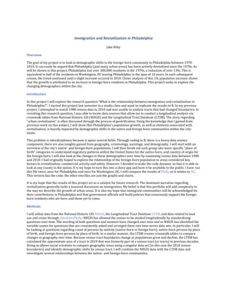
  • 12. #Creates columns to look at change in each census tract between 1980-2010 Tracts80to10 <- TractSpread%>% mutate(d80to10NB=n2010NB-n1980NB)%>% mutate(d80to10FB=n2010FB-n1980FB)%>% select(trtid10,d80to10FB,d80to10NB)%>% mutate(Change=ifelse((d80to10FB>0 & d80to10NB>0),"Both Increase", ifelse(d80to10FB>0 & d80to10NB<=0,"FB Increase Only", ifelse(d80to10FB<=0 & d80to10NB>0,"NB Increase Only", ifelse(d80to10FB<0 & d80to10NB<0,"Both Decrease","-"))))) #Shows a scatter plot of tracts that have had increases, decreases or no change in the native-/foreign-born populations ggplot(Tracts80to10, aes(d80to10NB, d80to10FB, color=factor(Change)))+ geom_point()+ geom_abline(intercept = 0, slope = 0)+ geom_vline(xintercept=0)+ coord_fixed()+ theme_bw()+ ggtitle(paste("Change in Number of Native Born and Foreign Born Populations nin each Census Tract in ",CityName,"nbet ween 1980-2010 ",sep=""))+ theme(plot.title = element_text(hjust = 0,size=12))+ xlab("Change in Native Born Population") + ylab("Change in Foreign Born Population")+ guides(color=guide_legend(title=NULL)) #provides a table as.data.frame(table(Tracts80to10$Change))%>% mutate(Pct=round(Freq/sum(Freq),2))%>% kable() Var1 Freq Pct - 13 0.03 Both Decrease 99 0.26 Both Increase 72 0.19 FB Increase Only 178 0.46 NB Increase Only 26 0.07
  • 13. Analysis Knowing that both cities took a huge hit in the 1970s, I chose to compare census tracts between 1980-2010. The scatter plot above shows four quadrants. To the right and left of 0 on the x-axis is the growth and loss of the native born. To the top and bottom of zero on the y-axis is the growth and loss of the foreign born. Dots in the upper right corner represent census tracts that have had an increase in both populations between 1980-2010, and dots in the lower left have had a net loss for btoh groups. In Philadelphia, this chart shows that 46% of the tracts in the city have had an increase in the foreign-born population without an increase in the native-born population. This is in stark comparison to the 7% of tracts that have only had increases in the native born and 19% where there has been growth of both groups. It is noticable that over 25% of census tracts have seen reductions in both populations. DC is simlar. In DC, 55% of census tracts have had a net growth only for the foreign-born population. In addition, DC has a higher rate of tracts in which both populations grew (27%), and a much lower rate for where both populations decreased (14%). #This adds two columns to the Tracts80to10 table in order to arrange tracts by growth/loss DistGrowth<-Tracts80to10%>% arrange(desc(d80to10NB))%>% mutate(OrderNB=row_number())%>% arrange(desc(d80to10FB))%>% mutate(OrderFB=row_number()) #Shows the distribution of growth/loss of native-born population ggplot(DistGrowth, aes(x=OrderNB,y=d80to10NB))+ geom_bar(stat="identity",position="identity",fill="blue",color=NA, width=1.5)+ theme_bw()+ ggtitle(paste("Census Tracts Arranged from Most Growth to Most Loss in the nNative Born Population in ",CityName,"n between 1980-2010 ",sep=""))+ theme(plot.title = element_text(hjust = 0,size=12))+ ylab("Change in Native-Born Population")+ xlab("Census Tracts Arranged from Growth to Loss") #table of growth/loss for Native Born DistGrowth%>% mutate(NBDirection=ifelse(d80to10NB>0,"Growth",ifelse(d80to10NB<0,"Loss","-")))%>% group_by(NBDirection)%>% summarise(Total=sum(d80to10NB))%>% kable() NBDirection Total - 0 Growth 51219 Loss -283821
  • 14. #Shows the distribution of growth/loss of foreign-Born population ggplot(DistGrowth, aes(x=OrderFB,y=d80to10FB))+ geom_bar(stat="identity",position="identity",fill="orange",color=NA, width=1.5)+ theme_bw()+ ggtitle(paste("Census Tracts Arranged from Most Growth to Most Loss in the nForeign Born Population in ",CityName," nbetween 1980-2010 ",sep=""))+ theme(plot.title = element_text(hjust = 0,size=12))+ ylab("Change in Foreign-Born Population")+ xlab("Census Tracts Arranged from Growth to Loss") #table of growth/loss for Foreign Born DistGrowth%>% mutate(FBDirection=ifelse(d80to10FB>0,"Growth",ifelse(d80to10FB<0,"Loss","-")))%>% group_by(FBDirection)%>% summarise(Total=sum(d80to10FB))%>% kable() FBDirection Total - 0 Growth 87458 Loss -15938
  • 15. #Shows growth of Foreign Born Population given the distribution of the Native Born Population ggplot(DistGrowth, aes(x=OrderNB,y=d80to10NB))+ geom_bar(stat="identity",position="identity",fill="blue",color=NA, width=1.5)+ geom_bar(aes(y=d80to10FB), stat="identity",position="identity",fill="orange",color=NA, width=1)+ theme_bw()+ ggtitle(paste("Growth of Foreign Born Population (orange) given the nGrowth of the Native Born Population (blue) ni n ",CityName," between 1980-2010 ",sep=""))+ theme(plot.title = element_text(hjust = 0,size=12))+ ylab("Change in Native-Born Population")+ xlab("Census Tracts Arranged from Growth to Loss (of Native-Born)")
  • 16. #Shows growth of Native Born Population given the distribution of the Foreign Born Population ggplot(DistGrowth, aes(x=OrderFB,y=d80to10FB))+ geom_bar(stat="identity",position="identity",fill="orange",color=NA, width=1.5)+ geom_bar(aes(y=d80to10NB), stat="identity",position="identity",fill="blue",color=NA, width=1)+ theme_bw()+ ggtitle(paste("Growth of Native Born Population (blue) given the nGrowth of the and Foreign Born Population (orange) nin ",CityName," between 1980-2010 ",sep=""))+ theme(plot.title = element_text(hjust = 0,size=12))+ ylab("Change in Foreign-Born Population")+ xlab("Census Tracts Arranged from Growth to Loss (of Foreign-Born)") #Linear model summary(lm(d80to10NB~d80to10FB, data=DistGrowth)) ## ## Call: ## lm(formula = d80to10NB ~ d80to10FB, data = DistGrowth) ## ## Residuals: ## Min 1Q Median 3Q Max ## -6299.8 -606.1 192.3 615.2 2908.6 ## ## Coefficients: ## Estimate Std. Error t value Pr(>|t|) ## (Intercept) -605.75107 58.32585 -10.386 <0.0000000000000002 *** ## d80to10FB 0.03397 0.13308 0.255 0.799 ## --- ## Signif. codes: 0 '***' 0.001 '**' 0.01 '*' 0.05 '.' 0.1 ' ' 1 ## ## Residual standard error: 1042 on 386 degrees of freedom ## Multiple R-squared: 0.0001688, Adjusted R-squared: -0.002421 ## F-statistic: 0.06515 on 1 and 386 DF, p-value: 0.7987 Analysis These charts show the distribution of change from most growth to most loss for the native-born (blue) and the foreign-born (orange). Here, Philadelphia & DC appear similar: approximately one-quarter of census tracts have had an increase in the native-born population, and more than half of the tracts have had increases for the foreign-born. This is more prnounced in DC with more than 75% of tracts showing growth for the foreign-born. Plotting the foreign-born distribution over the native-born distribution in Philadelphia shows that there is not much of a correlation (p=0.799). In DC, however, there appears to be more of an influence. It appears that presence of one group has a small correlation with the other (R2=0.025, p=0.0323)
  • 17. Median Home Values One hypothesis about immigrant communities is that working-class immigrants move into areas where housing is more affordable. To test this, I read in the 2010 Median House Value data from the American Communty Survey and added columns for number of foreign- born (n2010FB), number of native-born (n2010NB), totoal population (TPop) and density of foreign-born (FBDensity=n2010FB/TPop). MHValue <- getURL("https://raw.githubusercontent.com/rjake/FinalProject/master/ACS_10_5YR_B25077_MedianHouseValue.csv")%> %read.csv(text=., header = TRUE, skip=1, stringsAsFactors = FALSE)%>% #read.csv("ACS_10_5YR_B25077_MedianHouseValue.csv", header = TRUE, skip=1, stringsAsFactors = FALSE)%>% as.data.frame() MHValueCity <- MHValue%>% select(Id2,Estimate..Median.value..dollars.)%>% filter(substr(Id2,1,5)==findFIPS)%>% rename(FIPS=Id2)%>% rename(MHValue=Estimate..Median.value..dollars.)%>% mutate(MHValue=as.numeric(gsub("-","0",.$MHValue)))%>% mutate(FIPS=as.character(FIPS))%>% left_join(select(TractSpread, trtid10, n2010NB, n2010FB), by=c("FIPS"="trtid10"))%>% mutate(TPop=n2010FB+n2010NB)%>% mutate(FBDensity=round((n2010FB/TPop),5))%>%#*100)%>% mutate(MHValue1000s = MHValue/1000) #scatter plot of the relationship ggplot(MHValueCity, aes(FBDensity, MHValue1000s))+ geom_point()+ theme_bw()+ ggtitle(paste("Median House Value & Density of Foreign-Born Population n in ",CityName," (2010) ",sep=""))+ theme(plot.title = element_text(hjust = 0,size=12))+ xlab("% of Population that is Foreign-Born") + ylab("Median Home Value (Thousands)")
  • 18. #Linear Regression between Median House Value & Density of Foreign Born in 2010 summary(glm(FBDensity~MHValue1000s, family=binomial(logit),data=filter(MHValueCity, (n2010FB>0)& (MHValue>0)))) ## ## Call: ## glm(formula = FBDensity ~ MHValue1000s, family = binomial(logit), ## data = filter(MHValueCity, (n2010FB > 0) & (MHValue > 0))) ## ## Deviance Residuals: ## Min 1Q Median 3Q Max ## -0.43018 -0.23156 -0.10689 0.08689 1.02528 ## ## Coefficients: ## Estimate Std. Error z value Pr(>|z|) ## (Intercept) -2.336262 0.297832 -7.844 0.00000000000000436 *** ## MHValue1000s 0.001480 0.001353 1.094 0.274 ## --- ## Signif. codes: 0 '***' 0.001 '**' 0.01 '*' 0.05 '.' 0.1 ' ' 1 ## ## (Dispersion parameter for binomial family taken to be 1) ## ## Null deviance: 29.517 on 360 degrees of freedom ## Residual deviance: 28.383 on 359 degrees of freedom ## AIC: 93.317 ## ## Number of Fisher Scoring iterations: 5 Analysis Here I did find some relationship between the density of foreign born to median home value. Visually, I can see that, after the density of foreign-born people in a census tract in Philadlephia exceeds 30%, there becomes less variation in the median home values and the median value becomes closer to $200,000. I did not find statistically significant relationships between the two groups in either Philadelphia or DC. Mapping #Used following to create csv for Philadelphia shapefile #tract <- readOGR(dsn=".", layer="US_tract_2010", stringsAsFactors=FALSE) #tractCity <- tract[grepl(filterFIPS,tract$GEOID10),] #plot(tractCity) #fortify shapefile for use in ggplot # ggtract <- fortify(tractCity, region="GEOID10") # write.csv(ggtract,"ggtract.csv") ggtract <- getURL("https://raw.githubusercontent.com/rjake/FinalProject/master/ggtract.csv")%>%read.csv(text=., header = TRUE, stringsAsFactors = FALSE)%>% #read.csv("ggtract.csv", header = TRUE, stringsAsFactors = FALSE)%>% as.data.frame() #Table to create maps using standard deviations of population change DiffBoth <- TractSpread%>% mutate(id=as.numeric(trtid10))%>% #Values for Native Born mutate(d70to80NB=n1980NB-n1970NB)%>% mutate(d80to90NB=n1990NB-n1980NB)%>% mutate(d90to00NB=n2000NB-n1990NB)%>% mutate(d00to10NB=n2010NB-n2000NB)%>% #Values for Foreign Born mutate(d70to80FB=n1980FB-n1970FB)%>% mutate(d80to90FB=n1990FB-n1980FB)%>% mutate(d90to00FB=n2000FB-n1990FB)%>% mutate(d00to10FB=n2010FB-n2000FB)%>% select(id, starts_with("d")) %>% gather("Measure","Value", 2:9)%>% mutate(Decade=as.factor(substr(Measure,1,7)))%>% mutate(Pop=substr(Measure,8,9))%>% group_by(Pop)%>% mutate(SDValue=round(Value/sd(Value),2))%>% mutate(SD=cut(SDValue,breaks=c(-Inf,-3,-2,-1,1,2,3,Inf)))%>% left_join(.,ggtract) DiffBoth$Decade <- gsub("d70to80","1970-1980",DiffBoth$Decade) DiffBoth$Decade <- gsub("d80to90","1980-1990",DiffBoth$Decade) DiffBoth$Decade <- gsub("d90to00","1990-2000",DiffBoth$Decade) DiffBoth$Decade <- gsub("d00to10","2000-2010",DiffBoth$Decade) DiffBoth$Pop <- gsub("FB","Foreign-Born",DiffBoth$Pop) DiffBoth$Pop <- gsub("NB","Native-Born",DiffBoth$Pop)
  • 19. #Assign colors for standard deviation categories sd.fill <-c(brewer.pal(name="PuOr",n=7)[c(1,2,3)], "white", brewer.pal(name="PuOr",n=7)[c(5,6,7)]) sd.color <- c("gray45", "gray45", "gray45", "gray75", "gray45", "gray45", "gray45") #Goal: Function to map standard deviations in Philadelphia (convert to function?) #Steps: [fill] is dynamic as [SD] is a standardized column, #[element_blank()] removes axes labels #[scale_fill_manual] uses colors assigned to standard deviation (previous command) #Turn this into a function mapSD <- function(x) { ggplot(x)+ geom_polygon(aes(x=long, y=lat, group=group, fill=factor(SD),color=factor(SD)), size=0.1)+ theme(line=element_blank(), axis.text=element_blank(),axis.title=element_blank())+ scale_fill_manual(values=sd.fill,guide=guide_legend(reverse=TRUE))+ scale_color_manual(values=sd.color,guide=guide_legend(reverse=TRUE))+ coord_fixed()+ facet_grid(Pop~Decade)+ theme(panel.background=element_rect(fill="grey50")) } #Map Difference between decades using mapSD function above, facet wrap with 4 columns mapSD(DiffBoth)+ ggtitle(paste("Growth and Loss of Foreign-Born and Native-Born Population in n", CityName,"between 1980-2010 ",sep=""))+ theme(plot.title = element_text(hjust = 0,size=12))
  • 20. whichTracts<-Tracts80to10%>% mutate(id=as.numeric(trtid10))%>% filter(Change!="-")%>% left_join(.,ggtract) #Creates a map of locations that have had growth/loss for one or both groups ggplot()+ geom_polygon(data=ggtract, aes(x=long, y=lat, group=group), fill="white", color="grey70")+ geom_polygon(data=whichTracts, aes(x=long, y=lat, group=group, fill=Change))+ theme(line=element_blank(), axis.text=element_blank(),axis.title=element_blank())+ coord_fixed()+ facet_wrap(~Change, ncol=2)+ theme(panel.background=element_rect(fill="grey20"))+ ggtitle(paste("Growth and Loss of Foreign-Born and Native-Born Population in n", CityName," between 1980-2010 ",sep=""))+ theme(plot.title = element_text(hjust = 0,size=12)) Analysis The maps for the native-born population in Philadelphia show that mthe majority of the people who left the city left from North Philadelphia and the area between Penn and Graduate Hospital. For the native-born, 1 standard deviation is approximately 700 people. The darkest orange on the map thus represents at least a loss of 2,000 people in each census tract of that color. For the foreign born, there are more tracts showing growth than loss. For the foreign-born (in Philadelphia), 1 standard deviation is about 200 people and the brightest purple for the foreign-born is approximately 625 people. DiffBoth%>% group_by(Pop)%>% summarise(Std.Dev.1=round(sd(Value)))%>% mutate(Std.Dev.2=Std.Dev.1*2)%>%
  • 21. mutate(Std.Dev.3=Std.Dev.1*3)%>% kable() Pop Std.Dev.1 Std.Dev.2 Std.Dev.3 Foreign-Born 204 408 612 Native-Born 707 1414 2121 DecadeChange <- unique(DiffBoth[,1:7])%>% mutate(Growth=Value>=0)%>% group_by(Pop,Growth,Decade)%>% summarise(Difference = sum(Value)) ggplot(DecadeChange, aes(Decade,Difference))+ geom_bar(stat="identity", position="identity", color="black", aes(fill=Growth))+ facet_wrap(~Pop)+ theme_bw()+ ggtitle(paste("Difference in Population Between Decades for Foreign- & nNative-Born Population in ",CityName,"n bet ween 1970-2010 ",sep=""))+ theme(plot.title = element_text(hjust = 0,size=12))+ scale_y_continuous(breaks = seq(-300000, 100000, by = 50000)) Shows the total loss and total growth between each decade for each group DecadeChange%>% spread(Decade, Difference)%>% kable() Pop Growth 1970-1980 1980-1990 1990-2000 2000-2010 Foreign-Born FALSE -31717 -21895 -8376 -13179 Foreign-Born TRUE 12855 18723 40866 55381 Native-Born FALSE -274334 -127242 -131348 -91233 Native-Born TRUE 32701 27499 32262 57460 Analysis The above chart and graph show the trends for the growth and loss for each group between each decade. The net-loss of the native-born has lessened each decade. For the tracts that have seen growth, there has been a significant increase in the number of native-
  • 22. born people between 2000 and 2010 census, however, the net-growth for the city still puts the native-born population in a deficit. The trend looks similar in DC, however, there the growth is much greater than the loss and results in a net growth for the city. Below are the net growth totals between each decade for each group DecadeChange%>% group_by(Pop,Decade)%>% summarise(Difference=sum(Difference))%>% spread(Decade, Difference)%>% kable() Pop 1970-1980 1980-1990 1990-2000 2000-2010 Foreign-Born -18862 -3172 32490 42202 Native-Born -241633 -99743 -99086 -33773 Analysis Similar to the opening charts, the charts show the changes in population size for each group between the decades. Conculsion Overall, this analysis provides insight into changing demographics in Philadelphia (and in theory across the country). There are many more questions I wanted to ask with the data and I would like to continue developing this project. Unfortunately, I am at the mercy of the census bureau and aggregate information and the storage capacity available to me on git-hub. I had difficulty using the original shapefile for this dataset because it is very large and I was unable to host it on git-hub. Therefore, I was only able to upload the fortified version of Philadelphia County (ggtract.csv). I attempted to use centroids and other spatial arrangements however, it was too difficult to do given the time restriction. Future iterations of the projecte might include analysis on questions such as English language proficiency, proximity to commercial areas, length of stay in the United States, and majority racial group in each census tract. I hope this project inspires other people to learn more about their cities and can be used as a catalyst for future research.