Download to read offline
![© 2022, IRJET | Impact Factor value: 7.529 | ISO 9001:2008 Certified Journal | Page 295
IMAGE SEGMENTATION AND ITS TECHNIQUES
Kesha Chavda1, Gauraja Deo2, Sakshi Dhanu3, Prof. Mohan Bonde4
1,2,3 Information Technology, Usha Mittal Institute of Technology, Mumbai, India
4Assistant Professor, Usha Mittal Institute of Technology, Mumbai, India
-------------------------------------------------------------------***--------------------------------------------------------------------
Abstract— In digital image processing and computer
vision, image segmentation is a process that involves
separating a wide variety of images into various
segments. The goal of this procedure is to simplify and
improve the representation of an image. The role of
image segmentation is very important in image
processing. The partitioning of an image into multiple
segments makes it easier for further process. Thus,
after completing the operations, the image will be re-
joined. Segmentation increases the accuracy of
recognizing the object in an image and reduces the loss.
Semantic segmentation and Instance segmentation are
the types of image segmentation established on the
problem we use image segmentation.
Index Terms— LSTM, SVR, Linear Regression,
Sentimental Analysis, Stock Market Prediction
I. INTRODUCTION
An image contains a lot of useful information.
Understanding the image and extracting information from
the image to accomplish something is an application of
digital image technology. Therefore, the start in
understanding the image is Image Segmentation. In
practice, it’s often not inquisitive about all parts of the
image, but just for some certain areas which have identical
characteristics. Image segmentation is a vital basis for
image recognition. It is based on the group to divide an
input image into a number of the same nature of the group
in order to obtain the area in which people are interested.
And it’s the idea behind Image Analysis and understanding
of Image Feature Extraction and Recognition. Image
Segmentation is a way to partition an image into numerous
segments (subgroups) that help in reducing the intricacy of
the image, hence making the analysis of the image easier.
Various algorithms are used to allocate a certain set of
pixels together to form an image. We are basically assigning
labels to the pixels by doing so. Pixels with the same tag fall
under a category where they have some or the other thing
familiar in them. Using these labels, we are able to specify
boundaries, draw lines, and separate the foremost required
objects in a picture from the remainder of the not-so-
important ones.
II. PROPOSED SYSTEM
The aim of this project is to compare various Image
Segmentation techniques with Machine Learning, using
OpenCV, NumPy, TensorFlow, Keras, Scikit-Image, Python
Image Library (Pillow/PIL), and other python libraries, that
would help detect and identify the objects present around
one’s surroundings and compare their results.
III. RELATED WORK
In [1], the K-mean technique was used to implement image
segmentation on the image. An RGB image was transformed
into l*a*b* colour space because the RGB image was very
large. They concluded that in the K-mean algorithm, the
number of clusters was very important. If the number of
clusters was very high or very low, then the result was not
so good. K-mean showed every cluster in a new window,
and it made it easier to analyse the image for further
information. In Köhler’s method [2], Adaptive thresholding
was one of the most frequently used techniques in many
applications because it was fast to evaluate and when
merged with previous filters, it gave sturdy decision rules
for pattern recognition. In [3], the proposed segmentation
system provided a complete solution for both unsupervised
and supervised segmentation of colour images built on
neural networks. In the system, unsupervised segmentation
was implemented by SOM-based colour reduction and SA-
based colour clustering. The supervised segmentation was
achieved by HPL learning and pixel classification. The
system proposed in [4], presented and compared different
criteria to optimize segmentation parameters, when
examples are available. They also exposed another way to
take advantage of ground truth, in changing the data space
before applying the segmentation algorithm. It was shown
that using this knowledge to guide the segmentation
enables to produce better results, even better than
manually produced segmentation by an expert. The paper
[5] mainly focused on the study of the soft computing
approach to edge detection for image segmentation. The
soft computing approaches namely, fuzzy-based approach,
Genetic algorithm-based approach, and Neural network-
based approach were applied on a real-life example image
of a nature scene and the results showed the efficiency of
image segmentation. In [6] they proposed a conceptually
easy, pliable, and general framework for object instance
segmentation. Their approach efficiently detected objects in
an image while at once generating a high-quality
segmentation mask for each instance by using Mask R-CNN.
Mask R-CNN extends Faster R-CNN by appending a branch
for predicting an object mask aligned with the existing
branch for bounding box recognition. The paper [7]
International Research Journal of Engineering and Technology (IRJET) e-ISSN: 2395-0056
Volume: 09 Issue: 05 | May 2022 www.irjet.net p-ISSN: 2395-0072](https://image.slidesharecdn.com/irjet-v9i563-220929064421-445ad09d/75/IMAGE-SEGMENTATION-AND-ITS-TECHNIQUES-1-2048.jpg)
![International Research Journal of Engineering and Technology (IRJET) e-ISSN: 2395-0056
Volume: 09 Issue: 05 | May 2022 www.irjet.net p-ISSN: 2395-0072
© 2022, IRJET | Impact Factor value: 7.529 | ISO 9001:2008 Certified Journal | Page 301
closer its membership is close to the precise cluster centre.
Clustering-based segmentation are primarily used for
pattern recognition and data analysis.
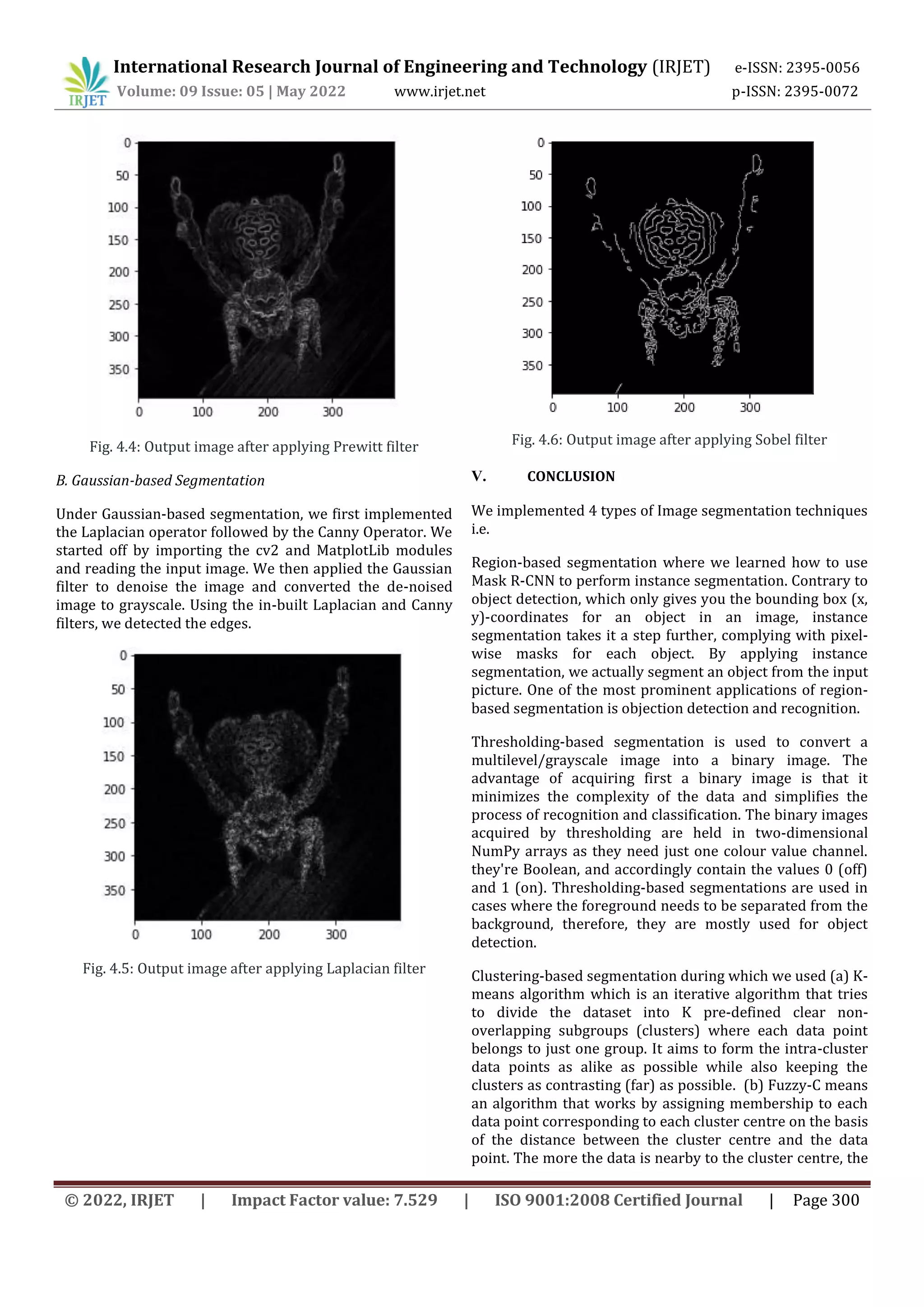
Edge-based segmentation remits to the process of
identifying and locating sharp discontinuities in an image.
The discontinuities are instantaneous changes in pixel
intensity that distinguish the boundaries of objects in a
scene. In this technique, we implemented the Sobel
Operator, Prewitt Operator, Canny Operator, and Laplacian
of Gaussian. From the experiment performed, it was
observed that the Canny result is the superior one when
compared to the other detectors for the selected image
since different edge detectors work better under different
conditions. Edge-based segmentation techniques are used
where finding out edges is important such as fingerprint
sensors.
VI. REFERENCES
[1] B. Tanwar, R. Kumar, and G. Gopal, ”Clustering
Techniques for Digital Image Segmentation”, vol. 7, no. 12,
pp. 55–60, 2016.
[2] Ralf Kohler, “A segmentation system based on
thresholding, Computer Graphics and Image Processing”,
Volume 15, Issue 4, ISSN 0146-664X, 1981.
[3] Guo Dong and Ming Xie, ”Learning for image
segmentation based on neural networks,” in IEEE
Transactions on Neural Networks, vol. 16, no. 4, pp., July
2005.
[4] I. Levner and H. Zhang, ”Classification-Driven
Watershed Segmentation,” in IEEE Transactions on Image
Processing, vol. 16, no. 5, pp., May 2007.
[5] N Senthilkumaran and Rajesh, Reghunadhan, “Edge
Detection Techniques for Image Segmentation - A Survey of
Soft Computing Approaches”, International Journal of
Recent Trends in Engineering, November 2007.
[6] Kaiming He, Georgia Gkioxari, Piotr Doll´ar, and Ross
Girshick,”Mask RCNN” ,IEEE International Conference on
Computer Vision (ICCV), 2017.
[7] P.Daniel Ratna Raju and G.Neelima, ”Image
Segmentation by using Histogram Thresholding”, 2012.
[8] K. Simonyan and A. Zisserman, ”Very deep convolutional
networks for largescale image recognition”, 2015.
[9] Kaiming He, Xiangyu Zhang, Shaoqing Ren, and Jian Sun,
“Deep Residual Learning for Image Recognition”, December
2015](https://image.slidesharecdn.com/irjet-v9i563-220929064421-445ad09d/75/IMAGE-SEGMENTATION-AND-ITS-TECHNIQUES-7-2048.jpg)

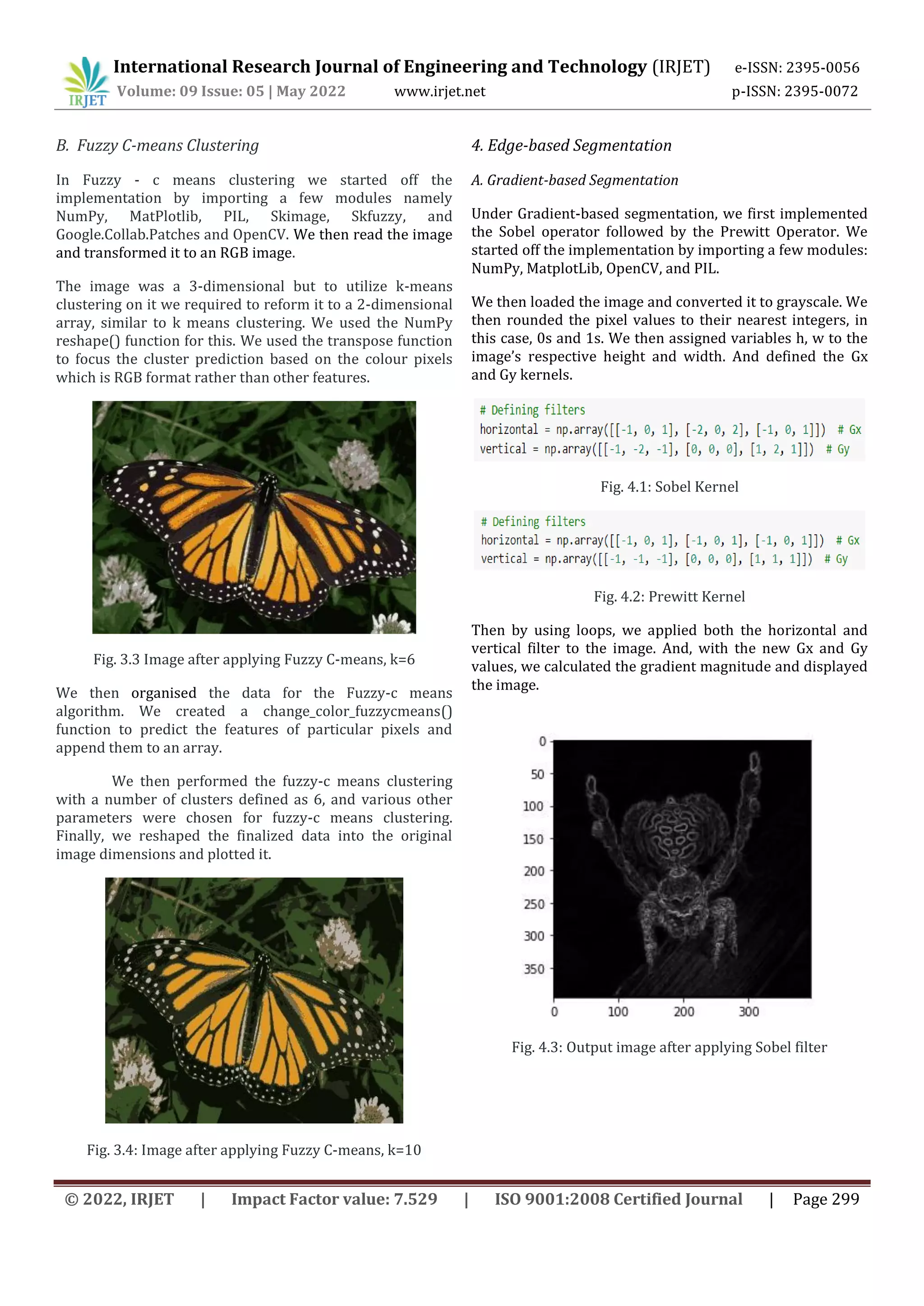
This document discusses various techniques for image segmentation. It begins with an abstract discussing image segmentation and its importance in image processing. It then discusses different types of image segmentation like semantic and instance segmentation. The document then discusses implementation of different image segmentation techniques. It implements region-based segmentation using Mask R-CNN. It performs thresholding-based segmentation using simple thresholding, Otsu's automatic thresholding. It also implements clustering-based segmentation using K-means and Fuzzy C-means. Furthermore, it implements edge-based segmentation using gradient-based techniques like Sobel and Prewitt, and Gaussian-based techniques like Laplacian and Canny edge detectors. Code snippets and output images are provided.