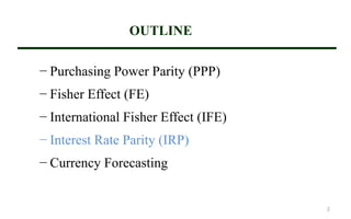
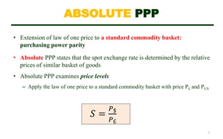
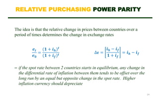
1) The document outlines several theoretical relationships between spot exchange rates, forward rates, inflation rates, and interest rates including purchasing power parity (PPP), the Fisher effect (FE), the international Fisher effect (IFE), and interest rate parity (IRP). 2) It discusses absolute and relative PPP, and that empirical tests show PPP holds better over the long-term than short-term and for countries with high inflation. 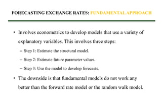3) The Fisher effect and international Fisher effect state that the difference in interest rates between countries should equal the difference in expected inflation rates.

1. TOPIC 4
PARITY CONDITIONS IN
INTERNATIONAL FINANCE &
CURRENCY FORECASTING
1

2. OUTLINE
− Purchasing Power Parity (PPP)
− Fisher Effect (FE)
− International Fisher Effect (IFE)
− Interest Rate Parity (IRP)
− Currency Forecasting
2

3. ARBITRAGE AND THE LAW OF ONE PRICE
FIVE KEY THEORETICAL RELATIONSHIPS AMONG SPOT RATE, FORWARD RATES,
INFLATION RATES, AND INTEREST RATES
Expected percentage
change of spot exchange
rate of foreign currency
- 3%
Expected inflation rate
differential
+ 3%
Forward discount or
premium on foreign
currency
- 3%
Interest rate
differential
+ 3%
FE
IFE
UFR
PPP
IRP

4. QUOTATION
Direct quote £1.00 = $2.00 ($: home currency, £: foreign currency)
Indirect quote $1.00 = £0.50
4

5. 5

6. 6

7. ABSOLUTE PPP
• Extension of law of one price to a standard commodity basket:
purchasing power parity
• Absolute PPP states that the spot exchange rate is determined by the relative
prices of similar basket of goods
• Absolute PPP examines price levels
– Apply the law of one price to a standard commodity basket with price P£ and PUS
7
𝑆 =
𝑃$
𝑃£

8. PPP AND EXCHANGE RATE DETERMINATION
Example, if an ounce of gold costs $2000 in the U.S. and
£1000 in the U.K., then the price of 1 £ in terms of dollars
should be:
Copyright © 2014 by the McGraw-Hill Companies, Inc. All rights reserved.
𝑆 =
𝑃$
𝑃£
=
$2000
£1000
= $2/£

9. https://www.economist.com/big-mac-index

10. 10

11. August 3, 2012
From The
Economist print
edition

12. BIG MAC INDEX - Burgernomics
12

13. IN-CLASS EXERCISE – 23.08.2022
13
https://www.economist.com/big-mac-index

14. RELATIVE PURCHASING POWER PARITY
The idea is that the relative change in prices between countries over a
period of times determines the change in exchange rates
– if the spot rate between 2 countries starts in equilibrium, any change in
the differential rate of inflation between them tends to be offset over the
long run by an equal but opposite change in the spot rate. Higher
inflation currency should depreciate
14
𝒆𝒕
𝒆𝟎
=
(𝟏 + 𝒊𝒉)𝒕
(𝟏 + 𝒊𝒇)𝒕
∆e =
𝒊𝒉 − 𝒊𝒇
𝟏 + 𝒊𝒇
= 𝒊𝒉 − 𝒊𝒇

15. RELATIVE PURCHASING POWER PARITY
Example: Price of a product is $100 in the US and ¥100 in Japan. For simplicity also
assume that exchange rate is $1.00/¥. Now suppose that due to inflation product’s price
increase to $110 in the US and to ¥105 in Japan (10% inflation in the US and 5% in
Japan). At the same time the new exchange rate is $1.02/¥. What are the implications of
these in terms of PPP?
Arbitrage is possible: Japanese product is relatively cheaper. A US based person now
needs $110 for the product if purchased in the US and only ¥105 x $1.02/¥ = $107.10 if
purchased in Japan. Therefore buy it in Japan spending $107.10 in dollars for purchase
and sell it in the US for $110. Your profit is $2.90. If exchange rate had changed to
$1.05/¥ (representing 5% inflation difference) then $ cost would be ¥105 x $1.05/¥ =
~$110.00
15

16. IN-CLASS EXERCISE
NĂM CPI-VN CPI-US NER
1992 100,0 100,0 10.800
1993 105,2 102,9
1994 114,4 101,8
1995 112,9 102,5
1996 105,5 102,5
1997 103,6 102,7 ???
16
𝑁𝐸𝑅𝑡 = 𝑁𝐸𝑅0
1 + 𝑖ℎ
𝑡
1 + 𝑖𝑓
𝑡

17. IN-CLASS EXERCISE
NĂM CPI-VN CPI-US RER
1992 100 100,0 10.800
1993 105,2 102,9
1994 114,4 101,8
1995 112,9 102,5
1996 105,5 102,5
1997 103,6 102,7 ???
17
𝑅𝐸𝑅𝑡 = 𝑅𝐸𝑅0
1 + 𝑖𝑓
𝑡
1 + 𝑖ℎ
𝑡

18. DOES PPP HOLD?
Empirical tests of both relative and absolute purchasing power parity show
that for the most part, PPP is not accurate in predicting future exchange rates
Reasons:
1. Price indexes not include non tradable goods
2. Goods baskets are not similar
3. Differential inflation rates might be inaccurate
4. Test periods are subject to government interventions
Two general conclusions can be drawn from the tests:
– PPP holds up well over the very long term but is poor for short term
estimates
– The theory holds better for countries with relatively high rates of
inflation and underdeveloped capital markets
18

19. THE FISHER EFFECT
• Fisher condition in U.S. and France: €
(1 + r$(Real)) = (1 + r$) / (1 + i$)
(1 + r€(Real)) = (1 + r€) / (1 + i€)
• If real rates are equal, then the Fisher condition implies:
• The difference in interest rates is equal to the expected difference in
inflation rates
19
f
h
f
h
i
i
r
r





1
1
1
1

20. INTERNATIONAL FISHER EFFECT – IFE
The International Fisher Effect, or Fisher-open, states that the
spot exchange rate should change in an amount equal to but in the
opposite direction of the difference in interest rates between
countries
20
t
f
t
h
t
r
r
=
e
e
)
1
(
)
1
(
0 


21. CURRENCY FORECATING
• Currency forecasting can lead to consistent profits only if the forecaster meets at least
one of the following four criteria.
– Has exclusive use of a superior forecasting model
– Has consistent access to information before other investors
– Exploits small, temporary deviations from equilibrium
– can predict the nature of government intervention in the foreign exchange
• As a general rule, in a fixed rate system, the forecaster must focus on the
governmental decision-making structure because the decision to devalue or revalue at
a given time is clearly political.
• In case of floating system, currency forecasting have the choice of using either
market or model-based forecasts, neither of which guarantees success.
21

22. EXHIBIT: EXCHANGE RATE FORECASTING IN PRACTICE
financial condition

23. FORECASTING EXCHANGE RATES: EFFICIENT MARKETS APPROACH
Financial markets are efficient if prices reflect all available and relevant
information.
− The efficient market hypothesis (Prof. Eugene Fama)
If this is true, exchange rates will only change when new information arrives,
thus:
St = E[St+1]
− The random walk hypothesis suggest that today’s ER is the best predictor of
tomorrow’s ER
Ft = E[St+1| It]
− Predicting exchange rates using the efficient markets approach is affordable and
is hard to beat.

24. FORECASTING EXCHANGE RATES: FUNDAMENTALAPPROACH
• Involves econometrics to develop models that use a variety of
explanatory variables. This involves three steps:
– Step 1: Estimate the structural model.
– Step 2: Estimate future parameter values.
– Step 3: Use the model to develop forecasts.
• The downside is that fundamental models do not work any
better than the forward rate model or the random walk model.

25. FORECASTING EXCHANGE RATES:
FUNDAMENTAL APPROACH
• S: natural logarithm of spot ER
• m-m*: natural logarithm of domestic/foreign money supply
•  - *: natural logarithm of domestic/foreign velocity of money
• y-y*: natural logarithm of domestic/foreign output
• : random error term, with zero mean
• , : model parameter






 






 )
(
)
(
)
( *
3
*
2
*
1 y
y
m
m
s

26. Data obtained from http://data.un.org
Inf_TK (%)
(1)
Inf_US (%)
(2)
∆Inf
(1)-(2)
S(TL/$)
End-of-year
rate
∆St/St-1 (%)
:= et
1989 0.0023
1990 60.3127 5.3980 54.9147 0.0029 26.6406
1991 65.9694 4.2350 61.7344 0.0051 73.3720
1992 70.0728 3.0288 67.0440 0.0086 68.5938
1993 66.0971 2.9517 63.1454 0.0145 68.9838
1994 106.2630 2.6074 103.6556 0.0387 167.5833
1995 88.1077 2.8054 85.3023 0.0597 54.0309
1996 80.3469 2.9312 77.4157 0.1078 80.6790
1997 85.7332 2.3377 83.3955 0.2056 90.7724
1998 84.6413 1.5523 83.0890 0.3145 52.9457
1999 64.8675 2.1880 62.6795 0.5414 72.1660
2000 54.9154 3.3769 51.5385 0.6734 24.3785
2001 54.4002 2.8262 51.5740 1.4501 115.3493
2002 44.9641 1.5860 43.3781 1.6437 13.3485
2003 25.2964 2.2701 23.0263 1.3966 -15.0307
2004 10.5842 2.6772 7.9070 1.3395 -4.0912
2005 10.1384 3.3928 6.7457 1.3451 0.4143
2006 10.5110 3.2259 7.2851 1.4090 4.7545
2007 8.7562 2.8527 5.9035 1.1708 -16.9056
2008 10.4441 3.8391 6.6050 1.5255 30.2913
2009 6.2510 -0.3555 6.6065 1.4909 -2.2649

27. Solution !
27

28. FORECASTING EXCHANGE RATES:
TECHNICAL APPROACH
• Technical analysis looks for patterns in the past behavior
of exchange rates.
• Clearly it is based upon the premise that history repeats
itself.

29. MOVING AVERAGE CROSSOVER RULE: GOLDEN CROSS vs DEATH CROSS
29
LMA: Long-term Moving Average SMA: Short-term Moving Average

30. HEAD AND SHOULDERS PATTERN: A REVERSAL SIGNAL
30

31. PERFORMANCE OF THE FORECASTERS
• Forecasting is difficult, especially with regard to the future.
• As a whole, forecasters cannot do a better job of
forecasting future exchange rates than the forecast implied
by the forward rate.
• The founder of Forbes Magazine once said, “You can
make more money selling financial advice than
following it.”

32. Chapter 4 32
)
(
)
(
F
MAE
S
MAE
R 
MAE(S): mean absolute forecast error of a forecasting service
MAE(F): mean absolute forecast error of the forward exchange rate as a predictor
 






 i i
i A
P
N
MAE
1

33. Chapter 4 33
)
(
)
(
S
MSE
B
MSE
R 
MSE(B): mean squared forecast error of a bank
MSE(S): mean squared forecast error of the spot exchange rate
MSE(B)<MSE(S): A bank provide more accurate forecast than spot ER, R<1

34. INVESTOR PSYCHOLOGYAND BANDWAGON EFFECTS
How are exchange rates influenced by investor psychology?
The bandwagon effect occurs when expectations on the part
of traders turn into self-fulfilling prophecies, and traders join
the bandwagon and move exchange rates based on group
expectations
• Governmental intervention can prevent the bandwagon from starting,
but is not always effective

35. 35
r
e
M
𝑴𝟐
𝒓𝟐
𝒆𝟐
𝒓𝟏
𝒆𝟏
𝑴𝟏
𝒓𝟑
𝑴𝟑
𝒆𝟑
ER, R AND MONEY SUPPLY