Download as PDF, PPTX


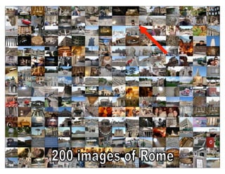

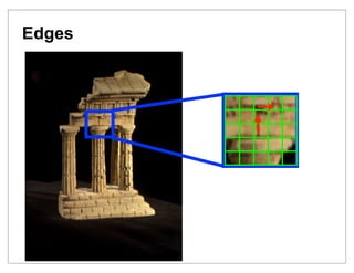
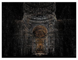
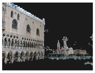
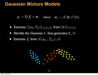
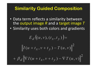
![Comparing images
Detect features using SIFT [Lowe, IJCV 2004]](https://image.slidesharecdn.com/icvss2011selectedprescomp-110903130024-phpapp02/85/ICVSS2011-Selected-Presentations-18-320.jpg)


![RBM predictedpredicted labels (47%)
RBM labels (47%)
Relation to other tasks sky sky
building building
tree
bed
tree
bed
car car
novel class
road road
Input search Ground truth neighbors
image image
Input Ground truth neighbors 32−RBM 32−RBM 16384-gist
1
query retrieved
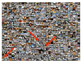
image retrieval object categorizationshowingitperce
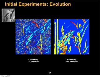
Figure 6. 6. Curves showing per
Figure Curves
query images that make it int
query images that make into
ofof the query for 1400 image
the query for a a 1400 imag
to 5% of the database size.
upup to 5% of the database siz
analogies: RBM predictedpredicted labels (56%)
RBM labels (56%) crucial for scalable retrieval th
crucial for scalable retrieval
- large databases tree
from [Nister and Stewenius, ’07]
tree sky sky
database make it it to the very
database make to the very to
is is feasible only for a tiny f
feasible only for a tiny fra
- efficient indexing database grows large. Hence, w
database grows large. Hence,
building building the curves meet the y-axis. T
the curves meet the y-axis.
- compact representation (a) car car given in in Table 1 for larger n
given Table 1 for a a larger
sidewalk sidewalkcrosswalkcrosswalk conclusions can bebe drawn from
conclusions can drawn from
road road improves retrieval performance
improves retrieval performan
differences: from neighbors et al., ’07] performance than vocabularies.1
performance than 2 -norm. En
L L2 -norm.
Input image imageGround truth [Philbinneighbors 32−RBM 32−RBM vocabularies. O
Input least for smaller 16384-gist
- simple notions of visual Ground truth least for smaller
gives much better performance th
gives much better performance
(b)
relevancy is is setting T.
setting T.
(e.g., near-duplicate,
same object instance, settings used by [17].
settings used by [17].
The performance with vav
The performance with
same spatial layout) (c)
RBM predictedpredicted labels (63%) [Torralba et al., ’08]
RBM labels (63%) from on the full 6376 image databa
on the full 6376 image data
the scores decrease with inc
the scores decrease with in
ceiling ceiling
are more images toto confus
are more images confuse
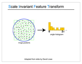
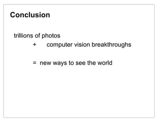
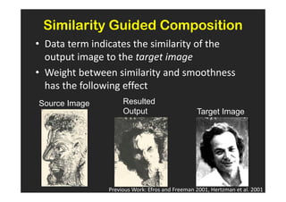
Figure Thewall retrieval performance is is evaluated using a large
wall performance evaluated using a large
Figure 5. 5. The retrieval ofof the vocabulary tree is sh
the vocabulary tree is show
ground truth database (6376 images) with groups ofof four images
ground truth database (6376 images) with groups four images
door door defining the vocabulary tree
defining the vocabulary tre
poster poster](https://image.slidesharecdn.com/icvss2011selectedprescomp-110903130024-phpapp02/85/ICVSS2011-Selected-Presentations-52-320.jpg)
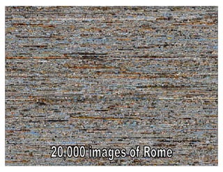
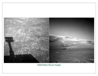
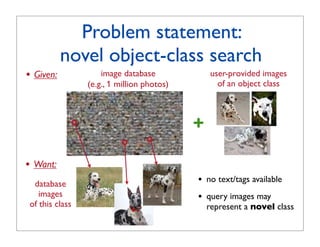
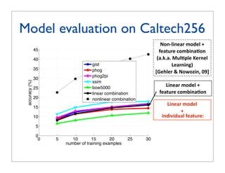
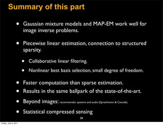
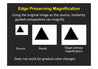
![State-of-the-art in
object classification
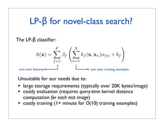
Winning recipe: many features + non-linear classifiers
(e.g. [Gehler and Nowozin, CVPR’09])
non-linear
!"#$%
decision boundary
!"#$%&#'()*
+&,-)&.&#(#/*
...
01#-2"#*
&'()*+),%%
-'.,()*+/%
#"0$%](https://image.slidesharecdn.com/icvss2011selectedprescomp-110903130024-phpapp02/85/ICVSS2011-Selected-Presentations-55-320.jpg)
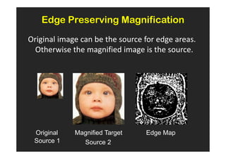
![m=1
s. For a kernel function k between a SVM.
he short-hand notation
Training Same as for averaging.
= k(fm (x), fm (x )),
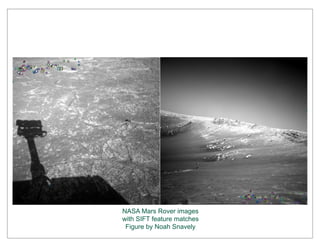
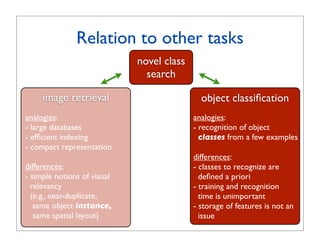
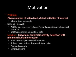
Multiple con- 4. Methods: Multiple Kernel Learning
kernel learning (MKL)
nel km : X × X → R only
espect to image feature fal., 2004; Sonnenburg etapproach toVarma and Ray, 2007] is to
[Bach et m . If the Another al., 2006; perform kernel selection
to a certain aspect, say, it only con- a kernel combination during the training phase of th
gorithm. jointly optimizing over
Learning a non-linear SVM by One prominent instance of this class is MKL
on, then the kernel measures simi-
F
a linear combinati
to this aspect. The subscript m of
nderstood as a linear combinationobjective ∗ (x, x ) k=(x, x ) =β over(x,fx ) x ) the par
1. indexing into the set of kernels k
is to optimize jointly
of kernels: ∗ F β k (x,
km f and
m
m=1 f =1
2. the SVM parameters: α ∈ RN and b ∈ R of an SVM.
ters
notational convenience, we will de- MKL was originally introduced in [1]. For efficiency
e of the m’th feature for a given
F in order N obtain sparse, F
to interpretable coefficients,
F
raining samples xi , i = 1, 1 . . . , N
min βf αT Kf α stricts βm ≥ 0 and ,imposes thefconstraintT α βm
+ C L yn b + β Kf (xn ) m=1
α,β,b 2 Since the scope of this paper is to access the applicab
f =1 n=1 f =1
of MKL to feature combination rather than its optimiz
), km (x, x2 ), . . . , km (x, xN )]T .
F part we opted to present the MKL formulations in a wa
aining sample, i.e. x = xi , then = 1,lowing for easier 1, . . . , F
subject to βf βf ≥ 0, f = comparison with the other methods
h column of the m’th kernel matrix.f =1 write its objective function as
F
ernel selection In this papert) = max(0, 1 − yt) 1
where L(y, we
min βm αT Km α
classifiers that aim to combine sev- 2 m=1
Kf (x) = [kf (x, x1 ), kf (x, x2 ), . . . , kf (x, xN )]T
α,β,b
e model. Since we associate image
N F
ctions, kernel combination/selection
+C L(yi , b + βm Km (x)T α)](https://image.slidesharecdn.com/icvss2011selectedprescomp-110903130024-phpapp02/85/ICVSS2011-Selected-Presentations-60-320.jpg)
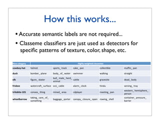
![LP-β: a two-stage approach to MKL
! [Gehler and Nowozin, 2009]
• Classification output of traditional MKL:
F
N
hM KL (x) = βf kf (x, xn )αn + b
f =1 n=1
• Classification function of LP-β:
F
N
h(x) = βf kf (x, xn )αf n + bf
f =1
n=1
hf (x)
Two-stage training procedure:
1. train each hf (x) independently → traditional SVM learning
2. optimize over β → a simple linear program](https://image.slidesharecdn.com/icvss2011selectedprescomp-110903130024-phpapp02/85/ICVSS2011-Selected-Presentations-61-320.jpg)
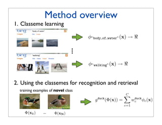
![Classemes: a compact descriptor for
efficient recognition [Torresani et al., 2010]
!
Key-idea: represent each image x in terms of its “closeness”
to a set of basis classes (“classemes”)
x
Φ(x) = [φ1 (x), . . . , φC (x)]T
F
N
φc (x) = hclassemec (x) = c
βf kf (x, xc )αn + bc
n
c
f =1 n=1
output of a pre-learned LP-β for the c-th basis class
Φ(x1 ) ... Φ(xN )
Query-time learning: training
examples of
train a linear classifier on Φ(x) novel class
C
F
N
g duck (Φ(x); wduck ) = Φ(x)T wduck = wc
duck c
βf kf (x, xc )αn + bc
n
c
c=1
f =1 n=1
LP-β trained before the
trained at query-time
creation of the database](https://image.slidesharecdn.com/icvss2011selectedprescomp-110903130024-phpapp02/85/ICVSS2011-Selected-Presentations-63-320.jpg)
![bject Classes by Between-Class Attribute Transfer
Hannes Nickisch Stefan Harmeling
Related work
or Biological Cybernetics, T¨ bingen, Germany
u
me.lastname}@tuebingen.mpg.de
•
otter
when train-
Attribute-based recognition:
black:
white:
yes
no
brown: yes
examples of stripes: no
hardly been water: yes
[Lampert et al., CVPR’09] [Farhadi et al., CVPR’09]
eats fish: yes
rule rather
ens of thou- polar bear
black: no
very few of white: yes
d annotated brown: no
stripes: no
water: yes
introducing eats fish: yes
ct detection zebra
ption of the black: yes
description white: yes
requires hand-specified attribute-class associations
brown: no
hape, color
s. On the left
h properties
stripes:
water:
yes
no
ribute be
hey can predic-
eats fish: no
to
displayed. attribute classifiers must be trained with
arethe cur- Figure 1. A description object categories: after learningthe transfer
by high-level attributes allows
ected based of knowledge between the visual
ed for a new cat- human-labeled examples
ve across appearance of attributes from any classes with training examples,
and to “engine”,can detect also object classes that do not have any training
ike facil- we based on which attribute description a test image fits best. randomly selected positively pre
new large- images, Figure 5: This figure shows
election helps
30,000 an- tributes for 12 typical images from 12 categories in Yahoo set.
nd “rein” that of well-labeled training imageslearnedtechniques
rson’s clas- lions and is likely out of
classifiers are numerous on Pascal train set and tested on Yahoo se
reach for years to come. Therefore,
emantic at-
one class outreducing the number of necessary training imagesattributes from the list of 64 attributes a
for domly select 5 predicted have](https://image.slidesharecdn.com/icvss2011selectedprescomp-110903130024-phpapp02/85/ICVSS2011-Selected-Presentations-65-320.jpg)
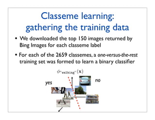
![Classeme learning:
choosing the basis classes
• Classeme labels desiderata:
- must be visual concepts
- should span the entire space of visual classes
• Our selection:
concepts defined in the Large Scale Ontology for Multimedia
[LSCOM] to be “useful, observable and feasible for automatic
detection”.
2659 classeme labels, after manual elimination of
plurals, near-duplicates, and inappropriate concepts](https://image.slidesharecdn.com/icvss2011selectedprescomp-110903130024-phpapp02/85/ICVSS2011-Selected-Presentations-67-320.jpg)
![Classeme learning:
training the classifiers
• Each classeme classifier is an LP-β kernel combiner
[Gehler and Nowozin, 2009]:
F
N
φ(x) = βf kf (x, xn )αf,n + bf
f =1 n=1
linear combination of feature-specific SVMs
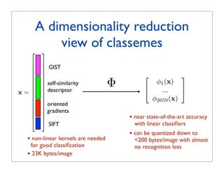
• We use 13 kernels based on spatial pyramid histograms
computed from the following features:
- color GIST [Oliva and Torralba, 2001]
- oriented gradients [Dalal and Triggs, 2009]
- self-similarity descriptors [Schechtman and Irani, 2007]
- SIFT [Lowe, 2004]](https://image.slidesharecdn.com/icvss2011selectedprescomp-110903130024-phpapp02/85/ICVSS2011-Selected-Presentations-69-320.jpg)
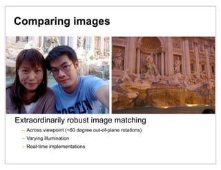
![Experiment 1: multiclass
recognition on Caltech256
60 LP-β in [Gehler
LPbeta Nowozin, 2009]
LPbeta13 using 39 kernels
50 MKL
Csvm LP-β with our x
Cq1svm
40 Xsvm our approach:
linear SVM with
accuracy (%)
classemes Φ(x)
30
linear SVM with
binarized classemes,
20 i.e. (Φ(x) 0)
linear SVM with x
10
0
0 10 20 30 40 50
number of training examples](https://image.slidesharecdn.com/icvss2011selectedprescomp-110903130024-phpapp02/85/ICVSS2011-Selected-Presentations-71-320.jpg)
![Accuracy vs. compactness
4
10
188 bytes/image
compactness (images per MB)
3
10
2.5K bytes/image
2
10
LPbeta13 23K bytes/image
1 Csvm
10
Cq1svm
nbnn [Boiman et al., 2008] 128K bytes/image
emk [Bo and Sminchisescu, 2008]
Xsvm
0
10
10 15 20 25 30 35 40 45
accuracy (%)
Lines link performance at 15 and 30 training examples](https://image.slidesharecdn.com/icvss2011selectedprescomp-110903130024-phpapp02/85/ICVSS2011-Selected-Presentations-73-320.jpg)

![Related work
• Prior work (e.g., [Sivic Zisserman, 2003; Nister Stewenius, 2006;
Philbin et al., 2007]) has exploited a similar analogy for
object-instance retrieval by representing images as bag of visual words
Detect interest patches Compute SIFT descriptors [Lowe, 2004]
…
…
Quantize
Represent image as a sparse
descriptors
histogram of visual words
frequency
…..
codewords
• To extend this methodology to object-class retrieval we need:
- to use a representation more suited to object class recognition
(e.g. classemes as opposed to bag of visual words)
- to train the ranking/retrieval function for every new query-class](https://image.slidesharecdn.com/icvss2011selectedprescomp-110903130024-phpapp02/85/ICVSS2011-Selected-Presentations-76-320.jpg)
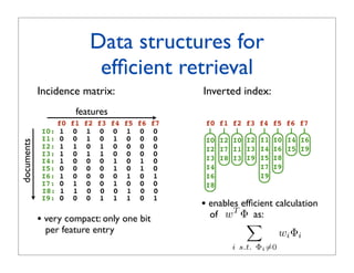
![Efficient retrieval via
inverted index
Inverted index:
w: [1.5 -2 0 -5 0 3 -2 0 ]
f0 f1 f2 f3 f4 f5 f6 f7
I0 I2 I0 I2 I1 I0 I4 I6
I2 I7 I1 I3 I4 I6 I5 I9
I3 I8 I3 I9 I5 I8
I4 I7 I9
I6 I9
I8
Goal:
compute score w T Φ, for all binary vectors Φ in the database
∀Φ](https://image.slidesharecdn.com/icvss2011selectedprescomp-110903130024-phpapp02/85/ICVSS2011-Selected-Presentations-78-320.jpg)
![Efficient retrieval via
inverted index
Inverted index:
w: [1.5 -2 0 -5 0 3 -2 0 ]
f0 f1 f2 f3 f4 f5 f6 f7
I0 I2 I0 I2 I1 I0 I4 I6
I2 I7 I1 I3 I4 I6 I5 I9
I3 I8 I3 I9 I5 I8
I4 I7 I9
I6 I9
I8
Scoring:
I0 I1 I2 I3 I4 I5 I6 I7 I8 I9](https://image.slidesharecdn.com/icvss2011selectedprescomp-110903130024-phpapp02/85/ICVSS2011-Selected-Presentations-79-320.jpg)
![Efficient retrieval via
inverted index
Inverted index:
w: [1.5 -2 0 -5 0 3 -2 0 ]
f0 f1 f2 f3 f4 f5 f6 f7
I0 I2 I0 I2 I1 I0 I4 I6
I2 I7 I1 I3 I4 I6 I5 I9
I3 I8 I3 I9 I5 I8
I4 I7 I9
I6 I9
I8
Scoring:
I0 I1 I2 I3 I4 I5 I6 I7 I8 I9](https://image.slidesharecdn.com/icvss2011selectedprescomp-110903130024-phpapp02/85/ICVSS2011-Selected-Presentations-80-320.jpg)
![Efficient retrieval via
inverted index
Inverted index:
w: [1.5 -2 0 -5 0 3 -2 0 ]
f0 f1 f2 f3 f4 f5 f6 f7
I0 I2 I0 I2 I1 I0 I4 I6
I2 I7 I1 I3 I4 I6 I5 I9
I3 I8 I3 I9 I5 I8
I4 I7 I9
I6 I9
I8
Scoring:
I0 I1 I2 I3 I4 I5 I6 I7 I8 I9](https://image.slidesharecdn.com/icvss2011selectedprescomp-110903130024-phpapp02/85/ICVSS2011-Selected-Presentations-81-320.jpg)
![Efficient retrieval via
inverted index
Inverted index:
w: [1.5 -2 0 -5 0 3 -2 0 ]
f0 f1 f2 f3 f4 f5 f6 f7
I0 I2 I0 I2 I1 I0 I4 I6
I2 I7 I1 I3 I4 I6 I5 I9
I3 I8 I3 I9 I5 I8
I4 I7 I9
I6 I9
I8
Scoring:
I0 I1 I2 I3 I4 I5 I6 I7 I8 I9](https://image.slidesharecdn.com/icvss2011selectedprescomp-110903130024-phpapp02/85/ICVSS2011-Selected-Presentations-82-320.jpg)
![Efficient retrieval via
inverted index
Inverted index:
w: [1.5 -2 0 -5 0 3 -2 0 ]
f0 f1 f2 f3 f4 f5 f6 f7
I0 I2 I0 I2 I1 I0 I4 I6
I2 I7 I1 I3 I4 I6 I5 I9
I3 I8 I3 I9 I5 I8
I4 I7 I9
I6 I9
I8
Scoring:
I0 I1 I2 I3 I4 I5 I6 I7 I8 I9](https://image.slidesharecdn.com/icvss2011selectedprescomp-110903130024-phpapp02/85/ICVSS2011-Selected-Presentations-83-320.jpg)
![Efficient retrieval via
inverted index
Inverted index:
w: [1.5 -2 0 -5 0 3 -2 0 ]
f0 f1 f2 f3 f4 f5 f6 f7
I0 I2 I0 I2 I1 I0 I4 I6
I2 I7 I1 I3 I4 I6 I5 I9
I3 I8 I3 I9 I5 I8
I4 I7 I9
I6 I9
I8
Cost of scoring is linear in the sum of the lengths of inverted
lists associated to non-zero weights](https://image.slidesharecdn.com/icvss2011selectedprescomp-110903130024-phpapp02/85/ICVSS2011-Selected-Presentations-84-320.jpg)
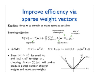
![Improve efficiency via
sparse weight vectors
Key-idea: force w to contain as many zeros as possible
classeme vector label of
Learning objective of example n example n
N
E(w) = R(w) + C
N n=1 L(w; Φn , yn )
regularizer loss function
• L2-SVM: R(w) = wT w , L(w; Φn , yn ) = max(0, 1 − yn (wT Φn ))
• L1-LR: R(w) = i |wi | , L(w; Φn , yn ) = log(1 + exp(−yn wT Φn ))
• FGM (Feature Generating Machine) [Tan et al., 2010]:
R(w) = wT w , L(w; Φn , yn ) = max(0, 1 − yn (w ⊙ d)T Φn )
s.t. 1T d ≤ B d ∈ {0, 1}D elementwise product](https://image.slidesharecdn.com/icvss2011selectedprescomp-110903130024-phpapp02/85/ICVSS2011-Selected-Presentations-86-320.jpg)
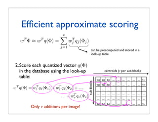
![Performance evaluation on
ImageNet (10M images)
35
! [Rastegari et al., 2011]
35
Full inner product evaluation L2 SVM
30
Full inner product evaluation L1 LR
30
Inverted index L2 SVM
Precision @ 10 (%)
25
Inverted index L1 LR
Precision @ 10 (%)
25
20
20 • Performance averaged over 400 object
15 classes used as queries
15 • 10 training examples per query class
10
10
• Database includes 450 images of the query
class and 9.7M images of other classes
5
5 •
Prec@10 of a random classifiers is 0.005%
0
20 40 60 80 100 120 140
Search time per query (seconds) 0
20 40 60 80 100 120 140
Each curve is obtained by varying sparsity through C in training objective Search time per query (seconds)
N
E(w) = R(w) + C
N n=1 L(w; Φn , yn )
regularizer loss function](https://image.slidesharecdn.com/icvss2011selectedprescomp-110903130024-phpapp02/85/ICVSS2011-Selected-Presentations-87-320.jpg)
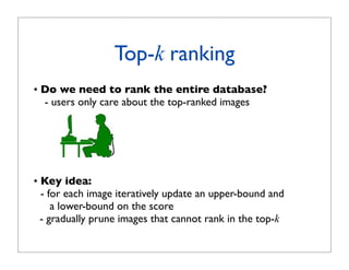
![Top-k pruning
! [Rastegari et al., 2011]
w: [ 3 -2 0 -6 0 3 -2 0 ]
• Highest possible score:
for binary vector ΦU s.t.
f0
I0: 1
f1
0
f2
1
f3
0
f4
0
f5
1
f6
0
f7
0
ΦU = 1 iff wi 0
i
I1: 0 0 1 0 1 0 0 0
I2: 1 1 0 1 0 0 0 0 → initial upper bound
I3: 1 0 1 1 0 0 0 0
I4: 1 0 0 0 1 0 1 0 u∗ = wT · ΦU (6 in this case)
I5: 0 0 0 0 1 0 1 0
I6: 1 0 0 0 0 1 0 1
I7: 0
I8: 1
1
1
0
0
0
0
1
0
0
1
0
0
0
0
• Lowest possible score:
I9: 0 0 0 1 1 1 0 1 for binary vector ΦL s.t.
ΦL = 1 iff wi 0
i
→ initial lower bound
l∗ = wT · ΦL (-10 in this case)](https://image.slidesharecdn.com/icvss2011selectedprescomp-110903130024-phpapp02/85/ICVSS2011-Selected-Presentations-89-320.jpg)
![Top-k pruning
! [Rastegari et al., 2011]
w: [ 3 -2 0 -6 0 3 -2 0 ] • Initialization: u∗ , l∗ for all images
upper bound
f0 f1 f2 f3 f4 f5 f6 f7
I0: 1 0 1 0 0 1 0 0
I1: 0 0 1 0 1 0 0 0
I2: 1 1 0 1 0 0 0 0
I3: 1 0 1 1 0 0 0 0
I4: 1 0 0 0 1 0 1 0
I5: 0 0 0 0 1 0 1 0 0
I6: 1 0 0 0 0 1 0 1
I7: 0 1 0 0 1 0 0 0
I8: 1 1 0 0 0 1 0 0
I9: 0 0 0 1 1 1 0 1
I0 I1 I2 I3 I4 I5 I6 I7 I8 I9
lower bound](https://image.slidesharecdn.com/icvss2011selectedprescomp-110903130024-phpapp02/85/ICVSS2011-Selected-Presentations-90-320.jpg)
![Top-k pruning
! [Rastegari et al., 2011]
w: [ 3 -2 0 -6 0 3 -2 0 ]
f0 f1 f2 f3 f4 f5 f6 f7
I0: 1 0 1 0 0 1 0 0
I1: 0 0 1 0 1 0 0 0
I2: 1 1 0 1 0 0 0 0 0
I3: 1 0 1 1 0 0 0 0
I4: 1 0 0 0 1 0 1 0
I5: 0 0 0 0 1 0 1 0
I6: 1 0 0 0 0 1 0 1
I7: 0 1 0 0 1 0 0 0
I8: 1 1 0 0 0 1 0 0
I9: 0 0 0 1 1 1 0 1
I0 I1 I2 I3 I4 I5 I6 I7 I8 I9
• Load feature i
• Since wi = +3 (0), for each image n:
- subtract +3 from the upper bound if φn,i = 0
- add +3 to the lower bound if φn,i = 1](https://image.slidesharecdn.com/icvss2011selectedprescomp-110903130024-phpapp02/85/ICVSS2011-Selected-Presentations-91-320.jpg)
![Top-k pruning
! [Rastegari et al., 2011]
w: [ 3 -2 0 -6 0 3 -2 0 ]
f0 f1 f2 f3 f4 f5 f6 f7
I0: 1 0 1 0 0 1 0 0
I1: 0 0 1 0 1 0 0 0
I2: 1 1 0 1 0 0 0 0 0
I3: 1 0 1 1 0 0 0 0
I4: 1 0 0 0 1 0 1 0
I5: 0 0 0 0 1 0 1 0
I6: 1 0 0 0 0 1 0 1
I7: 0 1 0 0 1 0 0 0
I8: 1 1 0 0 0 1 0 0
I9: 0 0 0 1 1 1 0 1
I0 I1 I2 I3 I4 I5 I6 I7 I8 I9
• Load feature i
• Since wi = -2 (0), for each image n:
- decrement by 2 the upper bound if φn,i = 1
- increment by 2 the lower bound if φn,i = 0](https://image.slidesharecdn.com/icvss2011selectedprescomp-110903130024-phpapp02/85/ICVSS2011-Selected-Presentations-92-320.jpg)
![Top-k pruning
! [Rastegari et al., 2011]
w: [ 3 -2 0 -6 0 3 -2 0 ]
f0 f1 f2 f3 f4 f5 f6 f7
I0: 1 0 1 0 0 1 0 0
I1: 0 0 1 0 1 0 0 0
I2: 1 1 0 1 0 0 0 0 0
I3: 1 0 1 1 0 0 0 0
I4: 1 0 0 0 1 0 1 0
I5: 0 0 0 0 1 0 1 0
I6: 1 0 0 0 0 1 0 1
I7: 0 1 0 0 1 0 0 0
I8: 1 1 0 0 0 1 0 0
I9: 0 0 0 1 1 1 0 1
I0 I1 I2 I3 I4 I5 I6 I7 I8 I9
• Load feature i
• Since wi = -6 (0), for each image n:
- decrement by 6 the upper bound if φn,i = 1
- increment by 6 the lower bound if φn,i = 0](https://image.slidesharecdn.com/icvss2011selectedprescomp-110903130024-phpapp02/85/ICVSS2011-Selected-Presentations-93-320.jpg)
![Top-k pruning
! [Rastegari et al., 2011]
w: [ 3 -2 0 -6 0 3 -2 0 ]
f0 f1 f2 f3 f4 f5 f6 f7
I0: 1 0 1 0 0 1 0 0
I1: 0 0 1 0 1 0 0 0
I2: 1 1 0 1 0 0 0 0 0
I3: 1 0 1 1 0 0 0 0
I4: 1 0 0 0 1 0 1 0
I5: 0 0 0 0 1 0 1 0
I6: 1 0 0 0 0 1 0 1
I7: 0 1 0 0 1 0 0 0
I8: 1 1 0 0 0 1 0 0
I9: 0 0 0 1 1 1 0 1
I0 I1 I2 I3 I4 I5 I6 I7 I8 I9
• Suppose k = 4:
we can prune I2,I9 since they cannot rank in the top-k](https://image.slidesharecdn.com/icvss2011selectedprescomp-110903130024-phpapp02/85/ICVSS2011-Selected-Presentations-94-320.jpg)
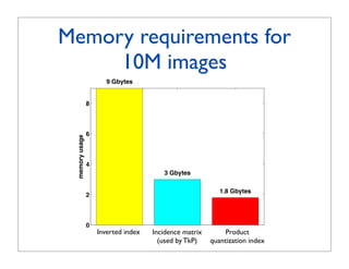
![Performance evaluation on 35
ImageNet (10M images) 30
35 ! [Rastegari et al., 2011]
Precision @ 10 (%)
25
30 TkP L1−LR
20
TkP L2−SVM
Inverted index L1−LR
Precision @ 10 (%)
25
15
Inverted index L2−SVM
20
10 • k = 10
15
• Performance averaged over 400 object
5 classes used as queries
10 • 10 training examples per query class
0
0 50 •
100 150 Database includes 450 images of the query
5 Search time per query (seconds) and 9.7M images of other classes
class
• Prec@10 of a random classifiers is 0.005%
0
0 50 100 150
Search time per query (seconds)
Each curve is obtained by varying sparsity through C in training objective
N
E(w) = R(w) + C
N n=1 L(w; Φn , yn )
regularizer loss function](https://image.slidesharecdn.com/icvss2011selectedprescomp-110903130024-phpapp02/85/ICVSS2011-Selected-Presentations-96-320.jpg)
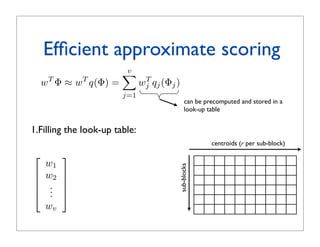
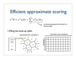
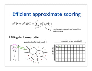
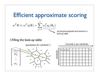
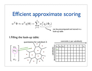
![Alternative search strategy:
approximate ranking
• Key-idea: approximate the score function with a measure that can
computed (more) efficiently (related to approximate NN search:
[Shakhnarovich et al., 2006; Grauman and Darrell, 2007; Chum et al.,
2008])
• Approximate ranking via vector quantization:
wT Φ ≈ wT q(Φ) !
q(!)
where q(.) is a quantizer returning
the cluster centroid nearest to Φ
• Problem:
- to approximate well the score we need a fine quantization
- the dimensionality of our space is D=2659:
too large to enable a fine quantization using k-means clustering](https://image.slidesharecdn.com/icvss2011selectedprescomp-110903130024-phpapp02/85/ICVSS2011-Selected-Presentations-97-320.jpg)
![Product quantization
!
Product quantization for nearest neighbor search
[Jegou et al., 2011]
• Split feature vector ! into v subvectors: ! [ !1 | !2 | ... | !v ]
Vector split into m subvectors:
• Subvectors are quantized separately by quantizers
Subvectors are quantized separately by quantizers
q(!) = [ q1(!1) | q2(!2) | ... | qv(!v) ]
where each qi(.) is learned in a space of dimensionality D/v
where each is learned by k-means with a limited number of centroids
• Example from [Jegou vector split in 8 subvectors of dimension 16
Example: y = 128-dim
et al., 2011]:
! is a 128-dimensional vector split into 8 subvectors of dimension 16
16 components
16 components
y1 y2 y3 y4 y5 y6 y7 y8
!1 !2 !3 !4 !5 !6 !7 !8
xedni noitazitnauq tib-46
stib 8
256 ) 1 y( 1 q
q
) 2 y( 2 q
q2
) 3 y( 3 q
q3
)4y(4q
q4
)5y(5q
q5
)6y(6q
q6
)7y(7q )8y(8q
q7 q8
28 = 256
centroids 1
centroids
q1 q2
1 q3
1 q4
1 q5 q6 q7 q8
sdiortnec 1q 2q 3q 4q 5q 6q 7q 8q
652
q1(y1) q2(y2) q3(y3) q4(y4) q5(y5) q6(y6) q7(y7) q8(y8)
q1(!1) q2(!2) q3(!3) q4(!4)
1
1y 1 1 1 1
2y 1 3y 4y 5y q5(!5) q6(!6) q7(!7) q8(!8)
6y 7y 8y
8 bits
stnenopmoc 61
64-bit quantization index
8 bits
64-bit quantization index
61 noisnemid fo srotcevbus 8 ni tilps rotcev mid-821 = y :elpmaxE
hcae erehw sdiortnec fo rebmun detimil a htiw snaem-k yb denrael si](https://image.slidesharecdn.com/icvss2011selectedprescomp-110903130024-phpapp02/85/ICVSS2011-Selected-Presentations-98-320.jpg)
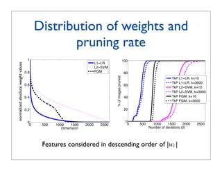
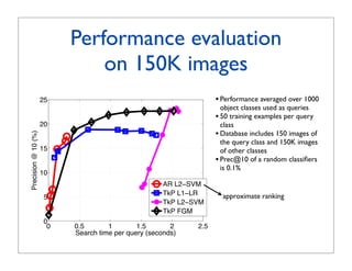
![Choice of parameters
! [Rastegari et al., 2011]
• Dimensionality is first reduced with PCA from D=2659 to D’ D
• How do we choose D’, v (number of sub-blocks),
r (number of centroids per sub-block)?
• Effect of parameter choices on a database of 150K images:
(v,r)
20
8 8
(128,2 ) (256,2 ) 6
(256,2 )
6
(64,2 )
15
Precision @ 10 (%)
6
8
(64,2 )
(32,2 )
(128,28)
D’=512
10 8
(16,2 ) D’=256
8 6
(32,2 ) (64,2 ) D’=128
5 (32,28)
8
(16,2 )
8
(16,2 )
0
0 0.05 0.1 0.15 0.2 0.25 0.3
Search time per query (seconds)](https://image.slidesharecdn.com/icvss2011selectedprescomp-110903130024-phpapp02/85/ICVSS2011-Selected-Presentations-105-320.jpg)
![Conclusions and open questions
Classemes:
• Compact descriptor enabling efficient novel-class recognition
(less than 200 bytes/image yet it produces performance similar to MKL
at a tiny fraction of the cost)
• Questions currently under investigation:
- can we learn better classemes from fully-labeled data?
- can we decouple the descriptor size from the number of
classeme classes?
- can we encode spatial information ([Li et al. NIPS10])?
• Software for classeme extraction available at:
http://vlg.cs.dartmouth.edu/projects/classemes_extractor/
Information retrieval approaches to large-scale object-class search:
• sparse representations and retrieval models
• top-k ranking
• approximate scoring](https://image.slidesharecdn.com/icvss2011selectedprescomp-110903130024-phpapp02/85/ICVSS2011-Selected-Presentations-108-320.jpg)


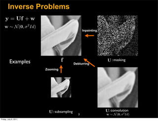
![Structured Sparsity
• PCA (Principal Component Analysis)
T
Σk = Bk S k Bk
• Bk = {φk }1≤m≤N PCA basis, orthogonal.
m
• Sk = diag(λk , . . . , λk ) , λk ≥ λk ≥ · · · ≥ λk eigenvalues.
1 N 1 2 N
• PCA transform
˜k = Bk ak
fi ˜i
• MAP with PCA
˜k = arg min Ui fi − yi 2 + σ 2 f T Σ−1 fi
fi ˜
i k
fi
⇔ N
|ai [m]|2
ak = arg min Ui Bk ai − yi 2 + σ 2
˜i
ai
m=1
λkm
22
Friday, July 8, 2011](https://image.slidesharecdn.com/icvss2011selectedprescomp-110903130024-phpapp02/85/ICVSS2011-Selected-Presentations-116-320.jpg)
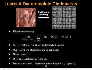
![Structured Sparsity
Sparse estimate v.s. Piecewise linear estimate
|Γ|
N
|ai [m]|2
2
ai = arg min UDai − yi + λ
˜ |ai [m]| ak
˜i 2
= arg min Ui Bk ai − yi + σ 2
ai ai λkm
m=1 m=1
D B1 B2 B3 B4 B5
• Linear collaborative filtering
Full degree of freedom
in each basis.
in atom selection |Λ|
|Γ|
• Nonlinear basis selection,
degree of freedom K.
23
Friday, July 8, 2011](https://image.slidesharecdn.com/icvss2011selectedprescomp-110903130024-phpapp02/85/ICVSS2011-Selected-Presentations-117-320.jpg)
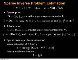
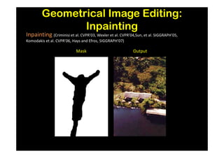
![Experiments: Inpainting
Original 20% available MCA 24.18 dB ASR 21.84 dB
[Elad, Starck, Querre, Donoho, 05] [Guleryuz, 06]
KR 21.55 dB FOE 21.92 dB BP 25.54 dB PLE 27.65 dB
[Takeda, Farsiu. Milanfar, 06] [Roth and Black, 09] [Zhou, Sapiro, Carin, 10]
26
Friday, July 8, 2011](https://image.slidesharecdn.com/icvss2011selectedprescomp-110903130024-phpapp02/85/ICVSS2011-Selected-Presentations-119-320.jpg)
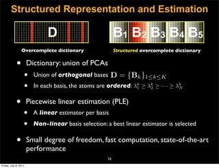
![Experiments: Zooming
Low-resolution
Original Bicubic 28.47 dB SAI 30.32 dB SR 23.85 dB PLE 30.64 dB
SR [Yang, Wright, Huang, Ma, 09] SAI [Zhang and Wu, 08]
29
Friday, July 8, 2011](https://image.slidesharecdn.com/icvss2011selectedprescomp-110903130024-phpapp02/85/ICVSS2011-Selected-Presentations-120-320.jpg)
![Experiments: Zooming Deblurring
f Uf y = SUf
Iy 29.40 dB PLE 30.49 dB SR 28.93 dB
[Yang, Wright, Huang, Ma, 09]
32
Friday, July 8, 2011](https://image.slidesharecdn.com/icvss2011selectedprescomp-110903130024-phpapp02/85/ICVSS2011-Selected-Presentations-121-320.jpg)
![Experiments: Denoising
Original Noisy 22.10 dB NLmeans 28.42 dB
[Buades et al, 06]
FOE 25.62 dB BM3D 30.97 dB PLE 31.00 dB
[Roth and Black, 09] [Dabov et al, 07]
34
Friday, July 8, 2011](https://image.slidesharecdn.com/icvss2011selectedprescomp-110903130024-phpapp02/85/ICVSS2011-Selected-Presentations-122-320.jpg)


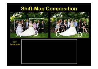
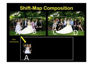
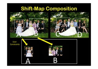
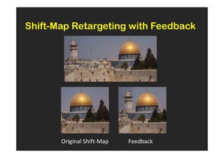
![Results and Comparison
Image completion with structure propagation [Sun et al. SIGGRAPH’05]
Shift-Map handles
without additional Mask Shift-Map
user interaction
some cases where
other algorithms
suggested that
can only be handled
with additional user
guidance
J. Sun, L. Yuan, J. Jia, and H. Shum. Image completion with structure propagation. In SIGGRAPH’05](https://image.slidesharecdn.com/icvss2011selectedprescomp-110903130024-phpapp02/85/ICVSS2011-Selected-Presentations-154-320.jpg)
![Results and
Comparison
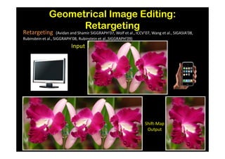
Non-Homogeneous Improved Seam Carving PatchMatch
[Wolf et al., ICCV’07] [Robinstein et al, SIGGRAPH’08] [Barnes et al, SIGGRAPH‘09]
Shift-Maps](https://image.slidesharecdn.com/icvss2011selectedprescomp-110903130024-phpapp02/85/ICVSS2011-Selected-Presentations-156-320.jpg)
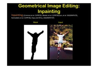
![The Bidirectional Similarity
[Simakov, Caspi, Shechtman, Irani – CVPR’2008]
Completeness All source patches
(at multiple scales)
source ⊆ target should be in the target
?
⊇ All target patches
(at multiple scales)
should be in the source
Coherence
Easy to compose (recover) source from target
Easy to compose (recover) target from source](https://image.slidesharecdn.com/icvss2011selectedprescomp-110903130024-phpapp02/85/ICVSS2011-Selected-Presentations-164-320.jpg)


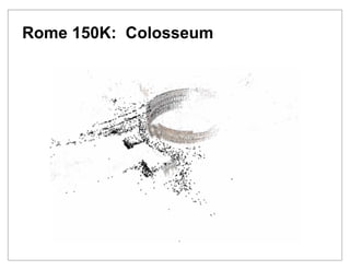
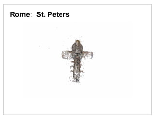
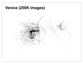
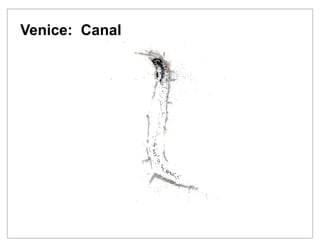
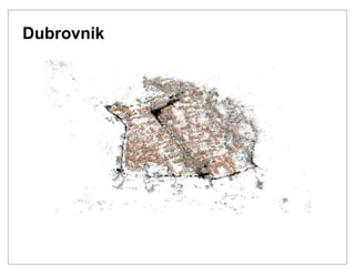
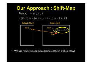
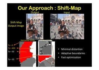
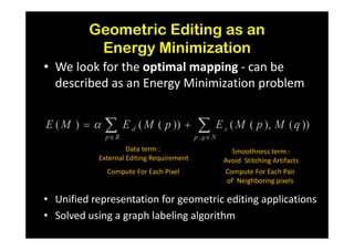
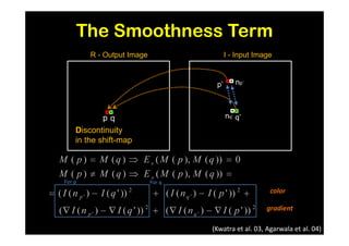
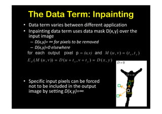
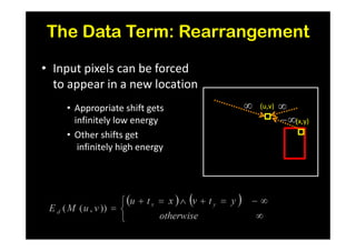
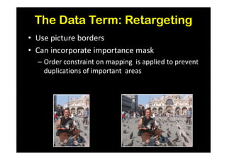
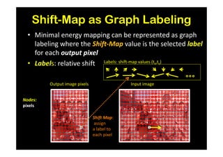
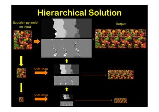
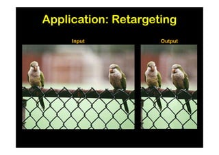
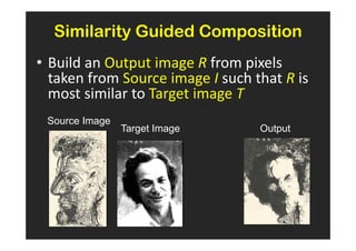
The document outlines the presentations from the International Computer Vision Summer School (ICVSS) 2011, featuring topics such as the handling and recognition of a trillion photos, efficient object-class recognition, and image rearrangement techniques. Notable speakers include Steven Seitz, Lorenzo Torresani, Guillermo Sapiro, and Shmuel Peleg, each discussing advancements in computer vision technology. The presentations highlight key methodologies for image comparison, classification, and search in large databases, as well as approaches to optimizing visual search tasks.


