Organizations using public cloud infrastructure are wise to deploy auto-scaling that adjusts server counts in response to sales volume fluctuations. We offer an approach for calculating the optimum minimal number of servers.

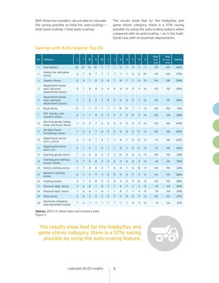
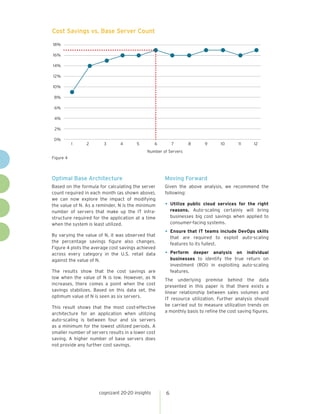
1. How Auto-Scaling Techniques
Make Public Cloud Deployments
More Cost-Effective
By moving to public cloud infrastructure, IT organizations can ap
auto-scaling techniques in which they pay only for the resources
are used. This can eliminate unused infrastructure during season
business slowdowns, resulting in significant cost savings.
ply
that
al
Executive Summary
Public cloud technologies have been widely
adopted by start-ups and small businesses due
to their low cost, flexibility and brief set-up time
required for the infrastructure. For larger estab-
lished enterprises, however, the infrastructure
set-up time is less of a concern, particularly
where private cloud hosting and virtualization
have reduced provisioning time considerably.
In such organizations, the smaller number of
benefits and concerns over data security have
meant that public cloud adoption has been less
forthcoming. This trend has been particularly
noted in the banking sector.
This white paper focuses on a key benefit
of public cloud hosting for larger and more
established enterprises that has largely gone
unnoticed: scalability.
The auto-scaling feature in Amazon Web Services
(AWS), in particular, allows elastic compute cloud
(EC2) instances to be scaled out automatically
following set rules around CPU, memory and
I/O utilization. For example, if a website needs
only two Web servers for 11 months of the year,
but 15 servers during the Christmas month, the
auto-scaling feature makes public cloud hosting
far less expensive than private cloud implemen-
tations. Traditional on-premises hosting would
have required the capacity of all 15 servers
throughout the year even when most of the
servers are not used. With auto-scaling in public
cloud, however, companies pay only for the
two servers for 11 months, which automatically
increases to 15 during the month of December
based on usage.
An analysis of U.S. Census retail data from 2015
shows a clear distinction in spending habits at
various times of the year. Retail customers who
shop in categories such as fuel dealers, and
hobby/toy and game stores spend over 220%
during the peak month of the year compared
with the lowest spending month. Traditional on-
premises hosting would result in tremendous
amounts of wasted IT resources, by reserving
capacity throughout the year to address peak
demand that corresponds with heavy usage
periods such as Thanksgiving, Black Friday,
Christmas and New Year’s.
cognizant 20-20 insights | november 2016
• Cognizant 20-20 Insights

2. cognizant 20-20 insights 2
The waste of computing resources is particu-
larly prevalent among those systems that handle
e-commerce, payment and back-end real-time
processing, such as stock tracking and accounts.
This paper also offers a snapshot of some such
systems in both the retail and retail banking
sectors.
By using the auto-scaling features of public
cloud, up to 57% in cost savings can be achieved
for such systems, on the assumption that there is
a linear correlation between spending amounts
and IT resource requirements. Analyzing the
savings trends also shows that the minimum
required server count for such applications
should be kept between four and six load-bal-
anced servers rather than a smaller number of
large servers.
The Capacity Management Problem
The capacity management problem has long
been a challenge for many enterprises. First,
there is a need to forecast the demand for new IT
resources based on future projects, and second,
there’s the need to optimize available resources
for systems that are already live. Much time and
resources are spent trying to forecast these two
requirements, and ensure that the optimum con-
figuration is ready to provision services quickly
and to reduce infrastructure resource waste.
Despite these efforts, the traditional on-premis-
es hosted IT service typically results in wasted
resources.
For the live systems, the peak workload is
estimated and resources set aside to meet this
demand at the most critical time frames. The
Christmas rush, for instance, is a key example
where retailers set aside large amounts of IT in
advance and in preparation for the big event.
In fact, research from Net Retail Federation
suggests that additional peaks during Black
Friday and Cyber Monday are starting to emerge,
and are likely to grow in the coming years.1
Similarly, in organizations where there is a large
amount of change, physical server capacity is
kept aside (e.g., for private cloud) to provision
virtual machines quickly and on demand when
required. Therein also lies potential waste where
it is practically impossible to have precisely the
right amount of physical hardware ready for
virtual machine provisioning.
This section explores the first of the two problems
noted above — which is the requirement for live
systems to predict utilization throughout the
year and set aside sufficient capacity to meet
peak demand.
The key data set used for carrying out this
analysis is 2015 U.S. Census retail data, which
in turn is based on the Monthly Retail Trade
Survey, Annual Retail Trade Survey and adminis-
trative records.2
The data reveals the estimated
monthly sales for various retail categories.
With this data as a starting point, the monthly
estimates were used to calculate the data
presented in Figure 1 (next page).
Our analysis shows that in some categories,
there was a 230% increase in monthly sales
volumes compared with the lowest month.
Translating this to IT, we assume that the
capacity of IT resources required to manage
sales volumes is linearly proportional to the
revenue recognized. Fuel dealers, for example,
will therefore need 230% more in IT resources
during peak months compared with lean sales
months.
By using the auto-scaling features of
public cloud, up to 57% in cost savings
can be achieved for such systems, on
the assumption that there is a linear
correlation between spending amounts
and IT resource requirements.
Fuel dealers, for example, will therefore
need 230% more in IT resources
during peak months compared with
lean sales months.

3. cognizant 20-20 insights 3
Therein lies the problem with traditional IT infra-
structure. Since IT infrastructure is dependent
on physical hardware which is time-consuming to
purchase and provision, huge amounts of wasted
resources are typically deployed to accommo-
date peak demand, which means much of the
infrastructure may lie fallow at other times of
the year.
IT Systems Related to Sale Volumes
Various core systems are likely to have a direct or
indirect impact on the fluctuating sale volumes
presented in Figure 1.
Figure 2 (next page) offers a cross-sectional view
of the systems used by retailers and banks that
are likely to have an impact on sales figures.
Front End
In retail, consumers start the buying process
through one of three channels — mobile, Web or
retail shops (either in a brick-and-mortar setting
or via telephone). These channels are typically
backed by a content management system and
portal, which includes Web, application and
database servers that can all benefit from
auto-scaling features. In the banking sector,
consumers interact and transact through their
Top 20 Estimates of Monthly 2015 Retail and Food Services Sales
by Business Type
Rank Category
Max
Month Sale
Min
Month Sale Max-Min % Diff
1 Fuel dealers 4,476 1,358 3,118 230%
2 Hobby, toy, and game stores 3,723 1,154 2,569 223%
3 Jewelry stores 5,807 1,841 3,966 215%
4 Department stores (excl. discount department stores) 9,257 3,493 5,764 165%
5 Department stores (excl. discount department stores) 9,623 3,639 5,984 164%
6 Book stores 1,633 690 943 137%
7 Gift, novelty, and souvenir stores 2,613 1,130 1,483 131%
8 Sporting goods, hobby, book, and music stores 12,897 5,716 7,181 126%
9 All other home furnishings stores 4,016 1,841 2,175 118%
10 Department stores (incl. L.D.)(3) 23,820 10,957 12,863 117%
11 Department stores (excl. L.D.) 23,425 10,797 12,628 117%
12 Sporting goods stores 6,209 2,870 3,339 116%
13 Clothing and clothing access. stores 33,123 15,733 17,390 111%
14 Family clothing stores 12,565 6,040 6,525 108%
15 Women’s clothing stores 4,984 2,537 2,447 96%
16 Clothing stores 22,884 11,649 11,235 96%
17 Discount dept. stores 14,168 7,297 6,871 94%
18 Discount dept. stores 14,197 7,312 6,885 94%
19 Shoe stores 3,938 2,029 1,909 94%
20 Electronic shopping and mail-order houses 55,765 29,879 25,886 87%
Category: These are the categories as provided in the U.S. Census retail data. Max Month Sale: This is the sales
volume, in millions of dollars, for the month that gave the highest sales in 2015. Min Month Sale: This is the sales
volume, in millions of dollars, for the month that gave the lowest sales in 2015. Max-Min: This column provides
the difference between the maximum and minimum sale months. % Diff: This column presents the Max–Min as
a percentage of the minimum sale month. This column essentially provides an estimate of monthly sales figure
disparities.
Note: Data for the top 20 categories was sorted based on the “% Diff” column.
Source: 2015 U.S. Retail Sales and Inventory Data
Figure 1

4. cognizant 20-20 insights 4
mobile, Web or internal core systems. These
systems are also likely to be utilized more heavily
during peak sales volumes.
Middle Tier
Following the front end, there is typically a tier
that handles the payments themselves. This is
usually shared between retailers (providing the
front end) and banks (providing the back end)
for processing the actual payments and trans-
actions. Such systems tend to work in real time3
that varies in utilization based on sales trends.
Back End
At the back end of retail organizations, numerous
real-time systems keep track of inventory and the
product purchase process. In banking, similarly,
there are back-end systems that keep track of
accounts and manage the transactions.
Savings Through Auto-Scaling
Using U.S. retail data, sales figures can be
mapped to the actual server capacity required
for each application tier to estimate the savings
achievable through auto-scaling.
With the monthly sales figures available for
each category, it is possible to extrapolate the
server count required for each month. Using
fuel dealers as an example, the month of August
saw the lowest sales figures. If we assume that
N servers are required to meet this demand in
August, then the server counts for the remaining
months can be extrapolated as a ratio of the
August sales using the following formula:
Server count for Month A = (N x Sales
for Month A) / Lowest Month Sales
Figure 3 (next page) provides the estimated
server count based on the above formula for
each of the 12 months in 2015 when N is assumed
to be six servers. Using these figures, the table
also calculates the total number of server
months required in 2015, based on auto-scaling,
and compares it with the total without auto-
scaling. The server count without auto-scaling
is estimated using the peak server month x 12
months (e.g., the maximum capacity required
in any month is assumed to be in place for all
months in the year).
Where Auto-Scaling Benefits Retail and Banking Systems
Retail
Mobile Store Web Mobile Bank Web
Banking
Shared Payment Processing Systems
Data Tier Back Office
Stock Control Accounts
Presentation Presentation
Figure 2Figure 2

5. With these two numbers, we are able to calculate
the saving possible as total (no auto-scaling) —
total (auto-scaling) / total (auto-scaling).
The results show that for the hobby/toy and
game stores category, there is a 57% saving
possible by using the auto-scaling feature when
compared with no auto-scaling — as is the tradi-
tional case with on-premises deployments.
cognizant 20-20 insights 5
The results show that for the hobby/toy and
game stores category, there is a 57% saving
possible by using the auto-scaling feature.
Savings with Auto-Scaling: Top 20
No. Category J F M A M J J A S O N D
Total
(Auto-
Scale)
Total
(No Auto-
Scale)
Saving
1 Fuel dealers 20 20 16 10 7 7 7 6 7 9 9 11 129 240 46%
2
Hobby, toy, and game
stores
6 7 8 7 7 7 7 7 7 8 12 20 103 240 57%
3 Jewelry stores 6 9 7 8 9 8 7 8 7 7 8 19 104 228 54%
4
Department stores
(excl. discount
department stores)
6 7 8 8 9 8 8 8 8 8 11 16 105 192 45%
5
Department stores
(excl. discount
department stores)
6 7 8 8 9 8 8 8 8 8 11 16 105 192 45%
6 Book stores 13 7 7 6 7 7 7 15 10 7 7 13 106 180 41%
7
Gift, novelty, and
souvenir stores
6 7 7 8 9 9 9 9 8 10 9 14 105 168 38%
8
Sporting goods, hobby,
book, and music stores
7 6 8 7 8 8 8 9 8 8 9 14 100 168 40%
9
All other home
furnishings stores
7 6 8 7 8 8 8 8 8 8 10 14 100 168 40%
10
Department stores
(incl. L.D.)(3)
6 7 8 7 8 7 7 8 7 8 10 14 97 168 42%
11
Department stores
(excl. L.D)
6 7 8 7 8 7 7 8 7 8 10 14 97 168 42%
12 Sporting goods stores 7 6 8 8 9 9 9 10 8 8 9 13 104 156 33%
13
Clothing and clothing
access. Stores
6 7 8 8 9 8 8 9 8 8 9 13 101 156 35%
14 Family clothing stores 6 7 8 8 8 7 8 8 7 8 18 13 106 156 32%
15
Women’s clothing
stores
6 7 9 9 9 8 8 9 8 9 9 12 103 144 28%
16 Clothing stores 6 7 9 8 9 8 8 9 8 9 10 12 103 144 28%
17 Discount dept. stores 7 6 8 7 8 7 7 8 7 7 9 12 93 144 35%
18 Discount dept. stores 7 6 8 7 8 7 7 8 7 7 9 12 93 144 35%
19 Shoe stores 6 8 9 8 9 8 9 11 8 8 9 12 105 144 27%
20
Electronic shopping
and mail-order houses
7 6 7 7 7 7 7 7 7 8 9 12 91 144 37%
Source: 2015 U.S. Retail Sales and Inventory Data
Figure 3

6. Optimal Base Architecture
Based on the formula for calculating the server
count required in each month (as shown above),
we can now explore the impact of modifying
the value of N. As a reminder, N is the minimum
number of servers that make up the IT infra-
structure required for the application at a time
when the system is least utilized.
By varying the value of N, it was observed that
the percentage savings figure also changes.
Figure 4 plots the average cost savings achieved
across every category in the U.S. retail data
against the value of N.
The results show that the cost savings are
low when the value of N is low. However, as N
increases, there comes a point when the cost
savings stabilizes. Based on this data set, the
optimum value of N is seen as six servers.
This result shows that the most cost-effective
architecture for an application when utilizing
auto-scaling is between four and six servers
as a minimum for the lowest utilized periods. A
smaller number of servers results in a lower cost
saving. A higher number of base servers does
not provide any further cost savings.
Moving Forward
Given the above analysis, we recommend the
following:
• Utilize public cloud services for the right
reasons. Auto-scaling certainly will bring
businesses big cost savings when applied to
consumer-facing systems.
• Ensure that IT teams include DevOps skills
that are required to exploit auto-scaling
features to its fullest.
• Perform deeper analysis on individual
businesses to identify the true return on
investment (ROI) in exploiting auto-scaling
features.
The underlying premise behind the data
presented in this paper is that there exists a
linear relationship between sales volumes and
IT resource utilization. Further analysis should
be carried out to measure utilization trends on
a monthly basis to refine the cost saving figures.
cognizant 20-20 insights 6
18%
16%
14%
12%
10%
8%
6%
4%
2%
0%
1 2 3 4 5 6 7 8 9 10 11 12
Number of Servers
Cost Savings vs. Base Server Count
Figure 4

7. About Cognizant
Cognizant (NASDAQ: CTSH) is a leading provider of information technology, consulting, and business process services,
dedicated to helping the world’s leading companies build stronger businesses. Headquartered in Teaneck, New Jersey
(U.S.), Cognizant combines a passion for client satisfaction, technology innovation, deep industry and business process
expertise, and a global, collaborative workforce that embodies the future of work. With over 100 development and
delivery centers worldwide and approximately 255,800 employees as of September 30, 2016, Cognizant is a member
of the NASDAQ-100, the S&P 500, the Forbes Global 2000, and the Fortune 500 and is ranked among the top per-
forming and fastest growing companies in the world. Visit us online at www.cognizant.com or follow us on Twitter:
Cognizant.
World Headquarters
500 Frank W. Burr Blvd.
Teaneck, NJ 07666 USA
Phone: +1 201 801 0233
Fax: +1 201 801 0243
Toll Free: +1 888 937 3277
Email: inquiry@cognizant.com
European Headquarters
1 Kingdom Street
Paddington Central
London W2 6BD
Phone: +44 (0) 20 7297 7600
Fax: +44 (0) 20 7121 0102
Email: infouk@cognizant.com
India Operations Headquarters
#5/535, Old Mahabalipuram Road
Okkiyam Pettai, Thoraipakkam
Chennai, 600 096 India
Phone: +91 (0) 44 4209 6000
Fax: +91 (0) 44 4209 6060
Email: inquiryindia@cognizant.com
­­© Copyright 2016, Cognizant. All rights reserved. No part of this document may be reproduced, stored in a retrieval system, transmitted in any form or by any
means, electronic, mechanical, photocopying, recording, or otherwise, without the express written permission from Cognizant. The information contained herein is
subject to change without notice. All other trademarks mentioned herein are the property of their respective owners.
Footnotes
1 Matthew Shay, “Black Friday: Changing, but far from gone,” Stores, National Retail Federation, December
16, 2015, https://nrf.com/news/black-friday-changing-far-gone.
2 “Annual Revision of Monthly Retail and Food Services: Sales and Inventories—January 1992 Through
March 2016,” U.S. Census, http://www.census.gov/retail/mrts/www/benchmark/2016/html/annrev16.
html.
3 “The Global Adoption of Real-Time Retail Payment Systems (RT-PS),” SWIFT 2015, https://www.google.
co.uk/url?sa=t&rct=j&q=&esrc=s&source=web&cd=1&ved=0ahUKEwiv68qerInNAhUlIcAKHXPuAlUQFg
gjMAA&url=https%3A%2F%2Fwww.swift.com%2Fnode%2F4716&usg=AFQjCNFG-0RiwEfZGpdOrajx7k
X_0sHzPw&sig2=uqZg9WKS6Sy_LCYTl8gmmg.
About the Authors
Naveen Thomas is a Senior Manager with Cognizant Infrastructure Services. He has over 12 years of
consulting experience at several leading consulting firms, focusing predominantly on innovation,
cloud technologies and infrastructure consulting. He holds a Ph.D. in computer vision and a master’s
degree in computer systems engineering from the University of Bristol. Naveen can be reached at
Naveen.Thomas@cognizant.com.
Alec Selvon-Bruce is a Director and Practice Lead for Enterprise Computing and Cloud Practice at
Cognizant Infrastructure Services in EMEA. He has over 22 years of professional services experience
across leading system integrations and technology providers. Alec drives the innovation councils that
provide guidance on infrastructure and cloud strategy. He holds a master’s degree in political studies
from the University Of Aberdeen. Alec can be reached at Alec.Selvon-Bruce@cognizant.com.
Codex 2050