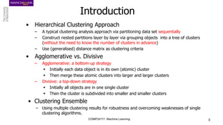
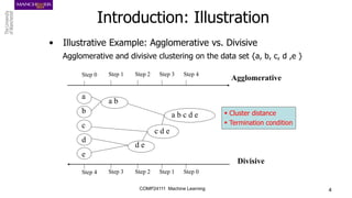
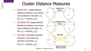
The document discusses hierarchical and ensemble clustering, detailing the agglomerative and divisive strategies used in clustering analysis. It covers key concepts such as distance measures, the agglomerative algorithm steps, and the lifetime of clusters, while also addressing the limitations of agglomerative methods and the benefits of clustering ensembles. Additionally, it highlights a clustering ensemble approach via evidence accumulation to improve robustness and performance in data analysis.

1. Hierarchical and Ensemble
Clustering
Ke Chen
Reading: [7.8-7.10, EA], [25.5, KPM], [Fred & Jain, 2005]
COMP24111 Machine Learning

2. COMP24111 Machine Learning 2
Outline
• Introduction
• Cluster Distance Measures
• Agglomerative Algorithm
• Illustrative example
• Key Concepts in Hierarchal Clustering
• Exercise
• Clustering Ensemble via Evidence Accumulation
• Summary

3. COMP24111 Machine Learning 3
Introduction
• Hierarchical Clustering Approach
– A typical clustering analysis approach via partitioning data set sequentially
– Construct nested partitions layer by layer via grouping objects into a tree of clusters
(without the need to know the number of clusters in advance)
– Use (generalised) distance matrix as clustering criteria
• Agglomerative vs. Divisive
– Agglomerative: a bottom-up strategy
 Initially each data object is in its own (atomic) cluster
 Then merge these atomic clusters into larger and larger clusters
– Divisive: a top-down strategy
 Initially all objects are in one single cluster
 Then the cluster is subdivided into smaller and smaller clusters
• Clustering Ensemble
– Using multiple clustering results for robustness and overcoming weaknesses of single
clustering algorithms.

4. COMP24111 Machine Learning 4
Introduction: Illustration
• Illustrative Example: Agglomerative vs. Divisive
Agglomerative and divisive clustering on the data set {a, b, c, d ,e }
 Cluster distance
 Termination condition
Step 0 Step 1 Step 2 Step 3 Step 4
b
d
c
e
a
a b
d e
c d e
a b c d e
Step 4 Step 3 Step 2 Step 1 Step 0
Agglomerative
Divisive

5. COMP24111 Machine Learning 5
single link
(min)
complete link
(max)
average
Cluster Distance Measures
• Single link: smallest distance
between an element in one cluster
and an element in the other, i.e.,
d(Ci, Cj) = min{d(xip, xjq)}
• Complete link: largest distance
between an element in one cluster
and an element in the other, i.e.,
d(Ci, Cj) = max{d(xip, xjq)}
• Average: avg distance between
elements in one cluster and
elements in the other, i.e.,
d(Ci, Cj) = avg{d(xip, xjq)}
d(C, C)=0

6. COMP24111 Machine Learning 6
Cluster Distance Measures
Example: Given a data set of five objects characterised by a single continuous feature, assume
that there are two clusters: C1: {a, b} and C2: {c, d, e}. (Minkowski distance for distance matrix)
1. Calculate the distance matrix . 2. Calculate three cluster distances between C1 and C2.
a b c d e
Feature 1 2 4 5 6
a b c d e
a 0 1 3 4 5
b 1 0 2 3 4
c 3 2 0 1 2
d 4 3 1 0 1
e 5 4 2 1 0
Single link
Complete link
Average
2
4}
3,
2,
5,
4,
min{3,
e)}
(b,
d),
(b,
c),
(b,
e),
(a,
d),
a,
(
,
c)
a,
(
min{
)
C
,
C
(
dist 2
1


 d
d
d
d
d
d
5
4}
3,
2,
5,
4,
max{3,
e)}
(b,
d),
(b,
c),
(b,
e),
(a,
d),
a,
(
,
c)
a,
(
max{
)
C
,
dist(C 2
1


 d
d
d
d
d
d
5
.
3
6
21
6
4
3
2
5
4
3
6
e)
(b,
d)
(b,
c)
(b,
e)
(a,
d)
a,
(
c)
a,
(
)
C
,
dist(C 2
1














d
d
d
d
d
d

7. COMP24111 Machine Learning 7
Agglomerative Algorithm
• The Agglomerative algorithm is carried out in three steps:
1) Convert all object features into
a distance matrix
2) Set each object as a cluster
(thus if we have N objects, we
will have N clusters at the
beginning)
3) Repeat until number of cluster
is one (or known # of clusters)
 Merge two closest clusters
 Update “distance matrix”

8. COMP24111 Machine Learning 8
• Problem: clustering analysis with agglomerative algorithm
Example
data matrix
distance matrix
Euclidean distance

9. COMP24111 Machine Learning 9
• Merge two closest clusters (iteration 1)
Example

10. COMP24111 Machine Learning 10
• Update distance matrix (iteration 1)
Example

11. COMP24111 Machine Learning 11
• Merge two closest clusters (iteration 2)
Example

12. COMP24111 Machine Learning 12
• Update distance matrix (iteration 2)
Example

13. COMP24111 Machine Learning 13
• Merge two closest clusters/update distance matrix
(iteration 3)
Example

14. COMP24111 Machine Learning 14
• Merge two closest clusters/update distance matrix
(iteration 4)
Example

15. COMP24111 Machine Learning 15
• Final result (meeting termination condition)
Example

16. COMP24111 Machine Learning 16
• Dendrogram tree representation
Key Concepts in Hierarchal Clustering
1. In the beginning we have 6
clusters: A, B, C, D, E and F
2. We merge clusters D and F into
cluster (D, F) at distance 0.50
3. We merge cluster A and cluster B
into (A, B) at distance 0.71
4. We merge clusters E and (D, F)
into ((D, F), E) at distance 1.00
5. We merge clusters ((D, F), E) and C
into (((D, F), E), C) at distance 1.41
6. We merge clusters (((D, F), E), C)
and (A, B) into ((((D, F), E), C), (A, B))
at distance 2.50
7. The last cluster contain all the objects,
thus conclude the computation
2
3
4
5
6
object
lifetime

17. COMP24111 Machine Learning 17
Exercise
Given a data set of five objects characterised by a single continuous feature:
The distance matrix on this dataset is given below. Apply the agglomerative algorithm with single-link,
complete-link and averaging cluster distance measures to produce three dendrogram trees, respectively.
a b C d e
Feature 1 2 4 5 6
a b c d e
a 0 1 3 4 5
b 1 0 2 3 4
c 3 2 0 1 2
d 4 3 1 0 1
e 5 4 2 1 0

18. COMP24111 Machine Learning 18
• Lifetime vs. K-cluster Lifetime
2
3
4
5
6
object
lifetime Key Concepts in Hierarchal Clustering
• Lifetime
The distance between that a cluster is created and that it
disappears (merges with other clusters during clustering).
e.g. lifetime of A, B, C, D, E and F are 0.71, 0.71, 1.41,
0.50, 1.00 and 0.50, respectively, the life time of (A, B) is
2.50 – 0.71 = 1.79, ……
• K-cluster Lifetime
The distance from that K clusters emerge to that K clusters
vanish (due to the reduction to K-1 clusters).
e.g.
5-cluster lifetime is 0.71 - 0.50 = 0.21
4-cluster lifetime is 1.00 - 0.71 = 0.29
3-cluster lifetime is 1.41 – 1.00 = 0.41
2-cluster lifetime is 2.50 – 1.41 = 1.09

19. COMP24111 Machine Learning 19
Relevant Issues
• How to determine the number of clusters
– If the number of clusters known, termination condition is given!
– The K-cluster lifetime as the range of threshold value on the dendrogram tree
that leads to the identification of K clusters
– Heuristic rule: cut a dendrogram tree at the maximum K-cluster life time to find a “proper” K
• Major weakness of agglomerative clustering methods
– Can never undo what was done previously
– Sensitive to cluster distance measures and noise/outliers
– Less efficient: O (n2 logn), where n is the number of total objects
• There are several variants to overcome its weaknesses
– BIRCH: scalable to a large data set
– ROCK: clustering categorical data
– CHAMELEON: hierarchical clustering using dynamic modelling

20. COMP24111 Machine Learning 20
Clustering Ensemble
• Motivation
– A single clustering algorithm may be affected by various factors
 Sensitive to initialisation and noise/outliers, e.g. the K-means is sensitive to initial centroids!
 Sensitive to distance metrics but hard to find a proper one
 Hard to decide a single best algorithm that can handle all types of cluster shapes and sizes
– An effective treatments: clustering ensemble
 Utilise the results obtained by multiple clustering analyses for robustness

21. COMP24111 Machine Learning 21
Clustering Ensemble
• Clustering Ensemble via Evidence Accumulation (Fred & Jain, 2005)
– A simple clustering ensemble algorithm to overcome the main weaknesses of
different clustering methods by exploiting their synergy via evidence accumulation
• Algorithm summary
– Initial clustering analysis by using either different clustering algorithms or running a
single clustering algorithm on different conditions, leading to multiple partitions
e.g. the K-mean with various initial centroid settings and different K,
the agglomerative algorithm with different distance metrics and forced to
terminated with different number of clusters…
– Converting clustering results on different partitions into binary “distance” matrices
– Evidence accumulation: form a collective “distance” matrix based on all the binary
“distance” matrices
– Apply a hierarchical clustering algorithm (with a proper cluster distance metric) to
the collective “distance” matrix and use the maximum K-cluster lifetime to decide K

22. Clustering Ensemble
 Example: convert clustering results into binary “Distance” matrix
A B
C
D
Cluster 1 (C1)
Cluster 2 (C2)













0
0
1
1
0
0
1
1
1
1
0
0
1
1
0
0
1
D
A D
C
B
D
C
A
B
“distance” Matrix
22
COMP24111 Machine Learning

23. Clustering Ensemble
Example: convert clustering results into binary “Distance” matrix
A B
C
D
Cluster 1 (C1)
Cluster 2 (C2)













0
1
1
1
1
0
1
1
1
1
0
0
1
1
0
0
2
D
A D
C
B
D
C
A
B
“distance Matrix”
23
Cluster 3 (C3)
COMP24111 Machine Learning

24. Clustering Ensemble
 Evidence accumulation: form the collective “distance” matrix
24













0
1
1
1
1
0
1
1
1
1
0
0
1
1
0
0
2
D













0
0
1
1
0
0
1
1
1
1
0
0
1
1
0
0
1
D















0
1
2
2
1
0
2
2
2
2
0
0
2
2
0
0
2
1 D
D
DC
COMP24111 Machine Learning

25. COMP24111 Machine Learning 25
Clustering Ensemble
 Application to “non-convex” dataset
– Data set of 400 data points
– Initial clustering analysis: K-mean (K=2,…,11), 3 initial settings per K  totally 30 partitions
– Converting clustering results to binary “distance” matrices for the collective “distance matrix”
– Applying the Agglomerative algorithm to the collective “distance matrix” (single-link)
– Cut the dendrogram tree with the maximum K-cluster lifetime to decide K

26. COMP24111 Machine Learning 26
Summary
• Hierarchical algorithm is a sequential clustering algorithm
– Use distance matrix to construct a tree of clusters (dendrogram)
– Hierarchical representation without the need of knowing # of clusters (can set
termination condition with known # of clusters)
• Major weakness of agglomerative clustering methods
– Can never undo what was done previously
– Sensitive to cluster distance measures and noise/outliers
– Less efficient: O (n2 logn), where n is the number of total objects
• Clustering ensemble based on evidence accumulation
– Initial clustering with different conditions, e.g., K-means on different K, initialisations
– Evidence accumulation – “collective” distance matrix
– Apply agglomerative algorithm to “collective” distance matrix and max k-cluster lifetime
Online tutorial: how to use hierarchical clustering functions in Matlab:
https://www.youtube.com/watch?v=aYzjenNNOcc