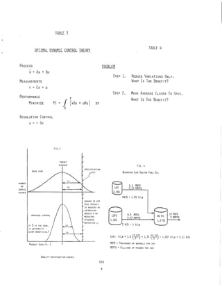
This document discusses the hidden economic benefits of improved process control that come from reducing quality variations, rather than just moving the average quality closer to specifications. It presents the typical approach of justifying process control investments based on improving the steady-state average. However, it argues this overlooks benefits from better dynamic performance. The document lays out the problem of relating dynamic control criteria to economic impacts, in order to properly assess the full financial benefits of reduced variations, not just improved averages.

1. I
tM. (v
76-528
THE HIDDEN BENEFITS FROM BETTER PROCESS CONTROL
Pierre R. Latour, Ph.D.
Biles & Associates
ISA~ IInternational Conference and Exhibit
Astrohall • Houston, Texas • October 11-14, 1976
Copyright 1976
In trument Society of America
400 Stanwix Street
Pitt burg , Pa. 15222

2. ©197G, ISA AC
THE HIDDEN BENEFITS FROM BETTER PROCESS CONTROL
Pierre R. Latour, Ph.D.
Manager, Process Control Engineering
Biles & Associates
P. O. Box 26125
Houston, Texas 77207
ABSTRACT
The improvements from better process
quality control are invariably perceived
in terms of steady state averages. Major
additional hidden benefits accrue from
dynamic concepts of reduced quality
variations alone. The theoretical foun-
dation is laid for assessing the economic
value of improved dynamic performance of
any process control system, giving a basis
for bridging the gap between modern con-
trol theory and industrial practice.
Important examples of application in
petroleum refining are cited.
INTRODUCTION
This paper is concerned with the methods
and techniques for establishing the eco-
nomic benefits from improved quality
control of manufactured products in gen-
eral. Our experience is oriented towards
the petroleum and chemical industries, so
we are principally concerned with improved
quality control 6f chemical products.
Very lar~~ investments are made for
improved process control, and these invest-
ments, both capital and expense, must be
justified based on an economic return.
Large sums are spent for process control
equipment listed in Table 1. In addition
to the equipment there are major expenses
for engineering, operations, and mainten-
ance of this equipment and for the people
responsible for process control and qual-
ity control. Our particular interest and
experience is in the area of economic
justification for on-line process control
computer systems. Invariably these must
be justified on the basis of improved
performance of the plant. This is mani-
fested in improved quality control and
hence, better yield of the most valuable
products, as well as reduced energy con-
sumption and operating costs and increased
plant capacity. It is well recognized
that justification of improved control
systems is a very difficult task, but it
is also very important. There are many
examples of remarkable payouts for improved
instrumentation and control systems, but
unfortunately there are too many examples
of poor investments as well. It is abso-
lutely essential to establish where the
benefits lie and where the biggest incen-
tives are in order to determine the empha-
sis and priority for designing comprehensive
computer and control systems.
NORMAL BENEFITS PROCEDURE
The typical criteria for product quality in
a petroleum refinery or chemical plant is
in terms of a quality specification limit.
Common examples of product specifications
are listed in Table 2. A product is deemed
to be satisfactory or acceptable if it is
within the specification and unacceptable
if it violates the specification. These
specification standards are typically
written in the legal contract for bulk
supplies to represent the performance of
the products manufactured in an industrial
plant.
The normal procedure for establishing the
benefits from improved process r.ontrol is
based on steady-state concepts(l,2,3). The
actual product quality will vary with time
as illustrated at the top of Figure 1.
This transient curve may represent the out-
put from an on-stream quality analyzer on
the product, or may represent a series of
bill~plevalues from laboratory analysis.
Naturally, if the analysis is of an inter-
mediate process stream, that goes to a
mixing tank, the variations must be atten-
uated to represent low frequency swings in
the final product where quality variations
have a meaningful economic influence. For
the given period of time, the quality meas-
urement is variable and has an average value
which is within the specification limit.
Values only approach or violate the speci-
fication on rare occasions. The improved
control system will reduce these fluctua-
tions in the product quality so that the
average value may be moved closer to
the specification without in fact violating
it. This is invariably the most profitable
52[;

3. SPEC
NUMBER
OF
SAMPLE
PO INTS 1--'=:"'---
FIG,2
FIG, 1
SPECIFICATION
LIMIT
~.
TARGET
AVERAGE
BASE CA3E
BASE CASE
Al
- - - - - -S" TARGET
AVERAGE
REDUCE FLUCTUATIONS
IMPROVED CONTROL
MOVE AVERAGE (SETPOINT) TOWARD SPEC
--;.- TIME
PRODUCT QUALITY, S
CONTROL QUALITY VARIATIONS WITH TIME
QUALITY DISTRIBUTION CURVES
TABLE 1
PROCESS CONTROL EQUIPMENT FOR PRODUCT QUALITY
TABLE 2
• STREAM ANALYZERS
• LABORATORY SAMPLING
TYPICAL EmlPLES FOR I1~PROVED QUALITY CONTROL
• INSTRUMENTATION 1. LOW.SULFUR FUEL OIL :<:::; l%wS
• CONTROL SYSTEMS 2, GASOLINE OCTANE 94 RONZ
• BLENDING SYSTEMS 3, HEAVY NAPHTHA ENDPOINT ~ 390'F
• SURGE TANKS 4, FUEL OIL VISCOSITY < 640 CSI122
• PROCESS COMPUTERS 5. CRUDE HEATER TEMPERATURE ~ 730'F
• AUTOMATION
6, DISTILLATION FLOODING < 100%
7, COMPRESSOR RPM < 6200
8, GAS OIL 90% POINT, ASHl D86 ~ 620'F
528
2

4. direction to move the product quality.
For example, in blending a low sulphur
fuel oi~ the closer the sulphur sp~cifi-
cations are approached the less the
requirement for the most valuable low
sulphur blending components. As gasoline
octane approaches a minimum specification
the gasoline yield or the operating cost
for adding lead anti-knock compounds
becomes more favorable. As the boiling
range of heavy naphtha from a crude dis-
tillation tower approaches its maximum
limit the yield of more valuable gasoline
increases. As fuel oil viscosity
approaches a maximum its yield or oper-
ating cost is more favorable. As the
temperature on a crude unit heater
approaches an upper limit the yield of the
most valuable products increases. As the
flooding point on a distillation column
is approached the column capacity
increases.
Therefore, the normal procedure for justi-
fying investments in improved process
control is invariably to estimate the
economic improvement by moving the average
value closer to the specification, and
this is a steady-state concept that really
relates to changing from the second curve
to the third curve in Figure 1. The
process control system is usually viewed
as a device that will allow that second
step by shrinking the transient variations
from the first to the second curve. In
fact, no economic benefits are credited
for that first step alone, based on
improved dynamic performance. Only the
second step of moving the average value
close to the specification is deemed to
give an economic benefit. The first step
is considered a necessary prerequisite.
This concept is often viewed in terms of
distribution functions for the data
collected over a period of time as indi-
cated in Figure 2. The upper curve
represents the distribution of quality
points about the average value or target
value and it indicates that a small
fraction of the data violates the speci-
fication limit. (If the limit is never
violated, the average or target is too
conservative.) The improved control case
shows data points clustered more closely
about the average value which has been
moved closer to the specification. If
the standard deviation, 0, is reduced by
a certain amount, the difference, ~,
between the limit and the target average
can be reduced by a corresp.onding amount.
This procedure of assessing the improve-
ment in the steady-state average quality
and assigning an economic benefit to that
improvement is probably the easiest way to
understand the improvements from process
control. However, it stands in sharp
contrast to the lessons of the technology
of modern optimal dynamic control theory
which has been developed over the last 15
years. Modern control theory teaches us
how to design feedback control systems
which will optimize the dynamic performance
of the plant with respect to a certain
dynamic performance criteria. The standard
nomenclature is listed in Table 3. The
first equation is a vector differential
equation that describes the process
dynamics of the plant in terms of the state
variables, x. The measured variables, Y,
are related to the state variables, X.
The performance index is an integral over
time of a quadratic formula for the state
variables, X and the control variables, U.
This is basically an integral squared
error type of performance index which is
to be minimized. State variables are
deviations about steady-state. The regu-
lation control formula would be a feedback
equation that gives the control variables,
U, in terms of the measurements, Y, or
state, X. Modern control theory allows
computation of the feedback gain matrix,
G, from the process and performance
matrices A, B, C, Q, and R. The question
that arises is how a dynamic performance
index can be related to process economics.
This is a modeling problem to evaluate the
parameters for Q and R in some way that is
meaningful to the economic performance of
the process plant. This has never been
done satisfactorily (5,6,7,8).
PROBLEM DESCRIPTION
The basic problem is to determine a clear
and direct way to relate dynamic criteria
to process economics. The problem can
be described by viewing two separate steps
indicated in Table 4. The first step is
to reduce the variations alone by improved
regulation about the same average value.
The question then arises, what is the net
benefit of this step alone? Is it zero?
Do the fluctuations really cancel out?
The second step is to move the average
value closer to the specification and
determine the net benefit of this step
alone. The difficult problem is evaluating
the first step. The contention of this
paper is that there is always economic
value associated with step one alone, but
establishing this benefit is often obscure
and difficult. This is the source of the
hidden benefits of improved quality control
that are invariably overlooked. In some
cases it can be shown that this hidden
benefit is quite significant.
The distribution curves for step one are
illustrated in Figure 3. In the improved
control case the standard deviation has
been reduced and the product is more uni-
form, but its average product quality is
unchanged. The problem is posed, is there
any benefit in improved product uniformity
528
3

5. TABLE 3
OPTIMAL DYNAMIC CONTROL THEORY
PROCESS
X = Ax + Bu
MEASUREMENTS
Y = Cx + D
PERFORMANCE
MINIMIZE PI
T
f [xQx + uRu 1
o
REGULATION CONTROL
U = - Gy
FIG.3
TARGET
AVERAGE
SPECIFICATION
[Mil
01
NUl'dlER
OF
SAMPLE
POINTS I-"'=--------+------t---=~
61
AMOUNT OF OFF
SPEC PRODUCT
[S REDUCED BY
[NCREAS [r<G
MARG [N 6 OR
REDUC[ NG
STANDARD
DEV[AT[ON 0,
[F S [S THE SANE.
[S UN[ FORMIlY
ALONE BENEF [C [AL?
PRODUCT QUAL! TY, S
QUAL!TY D[STR[BUTION CURVES
DT
528
PROBLEM
STEP 1.
STEP 2.
LSFO
1,1%S
TABLE 4
REDUCE VARIATIONS ONLY.
WHAT Is THE BENEFIT?
MOVE AVERAGE CLOSER To SPEC.
WHAT Is THE BENEFIT?
FIG, 4
BLEND[NG Low SULFUR FUEL OIL
1.1 MBPD
O. 33 t1~lPPD
4$/B = 1,33 ¢iLB
8,9 MBPD
2,67 MI1PPD
#6 Fa
1. 0 %S
"--- 3 $/B = 1 ¢iLB
COST, ¢ILB = 1.0 (2367) + 1.33 (~) = 1.037 ¢iLB = 3.11 $/B
I1BPD = THOUSANDS O~ BARRELS PER DAY
"lt1PPD = tlILLlONS OF POUNDS PER DAY
4

6. alone? Does the plant or the corporation
derive any economic benefit by virtue of
better product uniformity if the average
value is not moved closer to the specifi-
cation. We will show the answer is yes.
The first point to be observed is that the
amount of off-specification product in the
distribution tail is reduced by either
increasing the margin, 6, away from the
specification or by reducing the standard
deviation, 0, as occurs in the control
case. It is clear that if a model could
be derived for the economic penalty that
resulted from the specification violations
in the base case, one could determine the
improvements by virtue of the fact that
fewer samples violated the specification
after control was improved.
In the base case with a fixed, 01, consider
the problem of plant management in speci-
fying the best average target somewhat
within the specification limit. Certainly
one can imagine that if the target is far
below the limit there will be an important
economic loss, but as the target average
is moved closer and closer to the specifi-
cation limit the fraction off-specification
material produced begins to increase.
Clearly this will have an economic impact
on the long term plant performance. This
concept is built into the cornmon sense
statement, "It's better to play it on the
safe side." What this means is that the
true economic optimum point for the target
average is at some point which is offset
from the specification by 61, to trade off
yield benefits with customer dissatisfac-
tion. We will explore this concept with a
physical example in the next section,
FUEL OIL BLENDING EXAMPLE
Heavy No. 6 fuel oil is a major product of
petroleum refineries and is typically
burned in industrial and utility boilers
for generating steam and electricity. The
sulphur content specification is typically
less than 1% to insure satisfactory sulphur
dioxide emissions from the boiler to the
atmosphere. This fuel oil product is
usually made by the blending of two
components as illustrated in Figure 4.
One component will be a low sulphur fuel
oil (LSFO) slightly above the sulphur
specification. It will be upgraded with a
more valuable light gas oil (LGO) of low
sulphur content. The minimum amount of the
valuable LGO component will be used when
the final product is at its sulphur speci-
fication. If the product has less than
this sulphur content, too much LGO was used
with a resulting economic loss from quality
giveaway. For given prices the blending
components LGO and LSFO and their sulphur
content, a weight balance blending equation
will give the cost for producing the No. 6
fuel oil as indicated in Figure 4.
This equation is rewritten in general terms
of profit at the top of Figure 5. The
profit equation is plotted in Figure 5 in
terms of the quality of the product's
sulphur content. This steady-state equa-
tion applies for perfect quality control.
As the sulphur content of the product is
increasep the profit increases linearly,
and the maximum profit occurs when the
product is at the specification. A simple
calculation at the bottom of Figure 5
indicates the economic improvement by
moving the average sulphur content from
.95 to .98. The slope of this curve is
quite easy to determine from knowledge
about the manufacturing process. One can
imagine similar process relationships for
distillation columns, chemical reactors,
and almost any manufacturing operation.
We will continue to assume perfect control
in steady-state concepts. Now consider
what happens when a specification is not
made. This is illustrated in Table 5.
The profit still remains the selling price
minus the manufacturing cost but now we
must consider the selling price part of
the equation rather than the cost part.
Three particular situations are illus-
trated.
In one situation the product is worthless
when the specification is violated. The
selling price would be zero, and the profit
becomes negative. This would represent a
severe discontinuity in the profit equation
of Figure 5.
In the second situation, there might be a
sliding penalty on the selling price based
on the actual sulphur content of the
sample. This is typically the case for
No. 6 fuel oil which is shipped by ocean
tanker to the U. S. east coast. Upon
delivery it may be sampled by the customer
before acceptance. For example, if 2%
sulphur has one low price and 1% sulphur
has another higher price, a sliding scale
for the price per pound per percent sulphur
can be established and hence the actual
selling price is given by the equation with
the sliding penalty a function of the
degree the analysis exceeds the specifica-
tion. The actual profit equation expanded
to include this term is illustrated in
Table 5. These two terms for perfect
control are plotted in Figure 6. The
penalty term for reduced selling price
could be very severe and net profit drops
rapidly. Of course, the maximum profit
under perfect control is still achieved by
operating precisely at the specification.
A third situation can be treated where
repeated violations cause the plant to lose
customers. As production volume decreases,
some operating costs increase. For
example, Cl may increase as indicated by
the equation in Table 5. In this
528
5

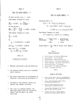
7. PROF IT
¢/LB
FIG, 5
PROF IT DEPENDS ~ QUALI TY
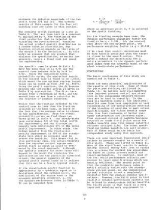
PROFIT = SELLING PRICE - COST
P = SP - C, ¢/LB
P = SP + (0 - ci) (~1-_5~2] - C2, C2> Cl
QUALITY,5
EXAMPLE CALCULAT I ON: AVERAGE SULFUR FROM 0.95 TO 0.98
AP = (C2 - ci) [~J -(C2 - ci ) [~JSl - S2 51 - 52
(C2 cr) [0.98 - 0.95] = (1.33 _ 1) [--.JWl.L....]Sl S2 1.1 - 0.2
AP = 0.0111 ¢iLB = 3. 3¢/B
Cl , COST OF LSoO, ¢/La
C2 c COST OF LGO, ¢ ILa
Sl " L500 SULFUR, ~
S2 c LGO SULFUR,
PROFIT
¢ILB
FIG, 6
SPEC VIOLATION PENALTY
SPO - a(S - SPEc) + (0 - ci) [~1-_S~2] - C2
PENALTY TERM COST TERM
/
/~
/ COST TERM
/
PENAL TY~-),
TERM
QUALITY, S
SPEC
TABLE 5
SUPPOSE THE SPECIFICATION II NOT MET
S > SPEC
PROFIT = SELLING PRICE - COST
P = SP' - C ¢/LB
CASE 1. WORTHLESS: SP = 0, SO P < 0
CASE 2, PENALTY: 2% 5 WORTH 2.41 $/B
1% 5 WORTH 3.11 $/B
70 ¢/B/%S = 0.233 ¢lLa/%s
SP = SPo - 0.233 (5 - SPEC)
P = SP 0 - a (5 - SPEel + (C2
) [L:....S.L] - C2- Cl 51 - 52
CASE 3, LOSE CUSTONERS: Cl INCREASES AT LmlER VOLUflE
Cl = Clo + P (S - SPEel , B> 0
C = (ClO - C2) [~SnJ + C2 + B(S - SPEC) [L-_5~2J
P = Sf> + (0 - Clo) [~l- _ SL] - C2 - ~ (i -S(S2+5PEC)+S2 SPEC)
FIG, 7
PROFIT DEPENDS ON AVERAGE QUALITY
PROFIT
¢ILB
BASE CASE
528
6

8. situation the profit equation becomes more
complex as a quadratic function of qual-
ity. These situations represent models
of the market and the economic environment
in which the commercial plant is oper-
ating. The best source of information for
these models is the legal contracts for
product sales to customers and marketing
studies.
HIDDEN BENEFITS FROM REDUCED VARIATIONS
Returning to Figure 6, we know that in
practice there is uncertainty in the
measurement and control of product quality
and the average target should be at some
safe value below the specification. A
realistic situation accounting for tran-
sients is sketched in Figure 7. Notice
this is a plot of actual profit versus
average or target quality. Given the
variability or distribution function in
the base case we know there must be some
economic penalty as the average is moved
closer to the limit, and the tail begins
to exceed the limit. In reality there
will be an optimum profit point as illus-
trated that is within the specification.
When we say in practice it is "better to
play it on the safe side," what we really
mean is that the maximum profit point
does not occur at the specification but
at a point within the specification. This
is because the economic penalty for vio-
lating the specification begins to become
significant and affect the overall
performance curve before the average value
reaches the limit, as illustrated. The
position of the penalty term depends on
the uniformity of product quality, 01.
This curve describes the profit of the
operation as a function of adjusting the
average quality target value closer to
the specification under a fixed control
system performance with a fixed distri-
bution curve and standard deviation, 01.
The improved control case is shown in
Figure 8. Here the variations have been
reduced and the average value can be
safely moved closer to the true speci-
fication. The optimum point is as
illustrated because the penalty term for
violating the specification does not
become significant until the average is
closer to the specification point. Notice
that this is a plot of profit versus the
average quality or target value, with a
fixed control system performance or a
fixed 02, less than 01.
These two curves are superimp9sed in
Figure 9. The first observation is that
the curve for the improved control case
has a different shape and has a different
long term steady-state profit function.
The second observation is that the actual
profit improvement from the best point
on the base curve to the best point on
on the improved control curve is the sum
of two components, ~Pl and ~P2. The
first component, ~Pl, is determined from
the slope of the cost portion of the curve
and the difference between the base optimum
target value and the improved optimum
target value. ~Pl represents a steady-
state cost benefit from moving the average
quality closer to the specification, Step 2
in Figure 1. This is the term that is the
most easily computed and one that is
commonly used for justification. The
second term, ~P2, is the fluctuation pen-
alty benefit that is derived from more
uniform quality alone at the same base
optimum average point. This is the hidden
component that is hard to quantify and is
always overlooked.
This profit benefit 6P2 is a real contrib-
utor to the plant profits. Where does the
money come from? This benefit money must
come from the fact that there are less
violations of the specification. If one
argues that in the base case there is no
violation of the specification, one is
saying that in the base case the operation
is far to the left of the base case optimum
point. This means there is an additional
benefit from moving up from that point to
the base optimum point by an operating cost
reduction. If the specification is never
violated, the target is not optimum. The
situation in Figure 9 is the conservative
evaluation because it assumes that the base
case operation is indeed operating at its
optimum point. The definition of this
smooth optimum is the point of tradeoff
between the cost curve and the economic
penalty curve for violating the specifi-
cation. Since the model of the specifica-
tion violation curve is so difficult to
obtain, it is usually neglected and the
component 6P2 is thereby also neglected.
Another observation in Figure 9 is that
as the standard deviation is reduced or
the control fluctuations are reduced the
shape of the steady long term profit
function changes. At constant average
quality, the profit increases by 6P2 from
the lower point to the middle point.
Since the profit function becomes narrower
the we i.qht i.nq factors in the dynamic per-
formance index in Table 3 would be changed
somewhat. Since the matrix Q is no longer
really a constant, this indicates that the
quadratic type performance index is not
strictly applicable. This is undoubtedly
due to the nonlinear nature of the penalty
functions. Perhaps in the unusual case
where the slope of the penalty curve is
symmetric with the slope of the cost curve,
the quadratic performance index would
apply.
FUEL OIL BLENDING CASE
An example problem was solved in detail to
528
7

9. PROFIT
¢iLB
FIG. S
PROFIT DEPENDS ON AVERAGE QUALITY
IMPROVED
CONTROL
TABLE 6
FUEL ill BLEND EXAMPLE -1
PROFIT = SELLING PRICE - OPERATING COST - Loss
P = SP - C - K1 (SPEC - S) - K2R
o
WHERE
K1 = ¢/LB/% SULF = 0,233
R = FRACTION REJECTED, DEPENDS ON ~/0
FROM CUMULATIVE PROBABILITY CURVE
K2 = ¢/LB COST INCURRED By VIOLATING
SPEC. REPROCESSING COST
528
8
PROF IT
¢iLB
m.9
IMPROVED CONTROL HAS A DIFFERENT
- --- PROFIT FUNCTION
/
/
/
IMPROVED
CONTROL
"Pi = STEADY STATE COST BENE;'IT FROM MOVING
AVERAGE QUALITY CLOSER TO SPECIFICATION
"P2 = FLUCTUATION PENALTY BENEFIT FROM MORE
UN I FORM PRODUCT QUAL! TY ALONE
TABLE 7
FUEL or L BLEND EXM1PLE - 2
SPEC = 1% SULF
BASE CASE SOPT = 0,95%
a1 = 0,99-0,95 = 0,04
a2 = 0,97-0,95 0,02
6.
1 = 0,95-1,0 = -0,05
~
a1
0,05 = -1.25
O~
COST
= K1
6.
K2 ~- t-
a a
AT OPTlfv1UM
d COST/a = K1 - K2 dR
10
0d6.ja d6.ja
a
dR
10
K1 ad6./a
R2

10. estimate the relative magnitude of the two
profit terms ~Pl and 6P2. The summary
results of this example for the fuel oil
blending case are given in this section.
The complete profit function is given in
Table 6. The last loss term is a constant
K2 multiplied by R, the fraction of the
total production that is rejected by
violating the specification. Assuming
the actual product quality distribution is
a random Gaussian distribution, the
fraction rejected depends on the ratio of
the margin 6 to the deviation o. In this
model we assumed that any product that
violates the specification, no matter how
severely, incurs a fixed cost per pound
for reprocessing.
The specific case is given in Table 7.
Here the base case 01 is 0.04 and the
control case reduces this by half to
0.02. Using the cumulative normal
probability curve, the equivalent margin
on the control case is found to be -.0343,
which means the new optimum average target
value can be moved up from .95% to .9657%.
Using the profit equation, the difference
between the two profit levels is given in
Table 8 by subtraction. The first term
arises from a reduction in cost, and the
second term arises from a reduction in
the fraction of product rejected.
Notice that the fraction rejected in the
control case is less than the fraction
rejected in the base case, in spite of
the fact that the average value is closer
to the specification. From the normal
probability curve, we find these two
terms given in Table 8. The steady-state
term contributes 53% of the total profit
for improvement, and the fluctuation
penalty term contributes 47% to the total
profit improvement. In other words, the
hidden benefit from the fluctuation
penalty improvement is 89% of the steady-
state term which is normally used to
assess the benefits. This means that in
this particular case, the actual benefits
from the improved control system are
almost twice as great as would be esti-
mated by the usual approach. Although
the specific results for other cases will
depend on the model for violating the
specification and the particular numerical
values, the general symmetry of the
optimum profit curves leads us to believe
that this may be a fairly typical result.
If the steady-state profit function is
approximated by a quadratic equation in
deviations about the optimum point, the
coefficient of the square term is the
economic weighting parameter, q, for
the dynamic performance index in Table 3.
It can be computed from
q
P -P
o ¢/lb
(%S)2(S-S )2
o
where an arbitrary point S, P is selected
on the profit function.
For the blending example base case, the
dynamic performance weighting factor was
found to be q = 3.388. For the control
case about the new optimum point, the
performance weighting factor is q = 10.928.
It is clear that control deviations must
be more heavily penalized when the target
is closer to the specification. This
gives a method for determining the Q
matrix parameters in the dynamic perform-
ance index from the economic model of the
plant steady-state performance.
CONCLUSIONS
The basic conclusions of this study are
summarized in Table 9.
There are many practical applications of
the results of this study. Some of these
for petroleum refining are listed in
Table 10. We believe many real benefits
from improved process control are often
lost in the intangible category because
they are so hard to quantify. In the
fuel oil blending example, the additional
benefits come from less complaints or less
reprocessing of off-specification material.
In the blending of gasoline to meet octane
specifications, the hidden benefit comes
from less lost customers or better cus-
tomer satisfaction and increased sales.
From improved control of naphtha/kerosene
cutpoint on crude distillation units the
hidden benefits come from longer catalytic
reformer catalyst life. The other speci-
fication hidden benefits are self evident.
Each of these would be the basis for
independent study using this approach.
There are some important theoretical impli-
cations to process control as a result of
this study. These are listed in Table 11.
Most of the significant results in modern
optimal control theory that lead to closed
form solutions for control law algorithms
are based on linear process models and
linear mathematics. In contrast, most of
the real world performance criteria are
encoded in legal specifications which are
heavily nonlinear. The second point is
that the quadratic performance index Q
matrix actually varies with the steady-
state average point, so the conventional
optimal criterion is not a completely
realistic form for process control appli-
cations. However, the third point is that
realistic dynamic performance criteria can
be related to steady-state dollar benefits.
The fourth point is that there is a very
important modeling work requirement to
528
9

11. TABLE 8
EUEL QlL BLEND EXAMPLE - 3
AT BASE OPTIMUM 61/°1 = - 1.25,
FROM NORMAL PROBABILITY CURVE
AT NEW
0.0913~§70 = = 0.1827
FROM NORMAL PROBABILITY CURVE
6
2 = -1. 715
°2
So
62 = -1.715(0.02) = -0.0343
NEW SOPT = 1-0.0343 = 0.9657%
BASE CASE SOPT = 0.9500%
R1 = 0.1056, R2 = 0.0431
TABLE 10
CON C L U S ION S
• REDUCED FLUCTUATIONS ALONE ARE BENEFICIAL
• THE IMPROVED CONTROL CASE HAS A DIFFERENT
PROFIT FUNCTION
• ONE SHOULD INVESTIGATE THE CONSEQUENCES OF
VIOLATING A SPECIFICATION AND QUANTIFY IT
THE BENEFITS FROM COMPUTER CONTROL ARE
GREATER THAN COMMONLY ESTIMATED
FOR A FUEL OIL BLENDING EXAMPLE, THE
ADDITIONAL BENEFIT FROM THE FLUCTUATION
PENALTY TERM WAS 89% OF THE STEADY
STATE TERM
TABLE 9
FUEL Qll BLEND EXAMPLE - 4
INCREASED PROFIT Is
P2-P1 = 6p = K1(62-61)-K2(R2-R1)
6p = K1(-0.0343 + 0.05) + K2(R1-R2)
= 0.0157 K1 + K101(R1-R2)/0.1827
FROM NORMAL PROBABILITY CURVE
6P = 0.0157 Kl + 0.0137 Kl = 0.0294K1
PROF IT
IMPROVEMENT
STEADY STATE
TERM
(53%)
FLUCTUA TION
PENALTY TERM
+ (47%)
+
HIDDEN BENEFIT = ~ 89% OF STEADY STATE BENEFIT
TABLE 11
PRACTICAL WPLI CAT! ONS
1. FUEL OIL SULFUR - LESS COMPLAINTS/REPROCESSING
2. GASOLI NE OCTANE - LESS LOST Cusrontns
3. NAPHTHA ENDPOINT - LONGER REFORr'lER CAT LIFE
4. FUEL OIL VISCOSITY - LESS COMPLAINTS/REPROCESSING
5. FURNACE TEr1PERATURE - LESS COKING, LONGER TUBE LIFE
6. DISTILLATION FLOODING - LESS OCCURENCE
7. COMPRESSOR RPM - LESS COMPRESSOR MAINTENANCE
8. GAS OIL - lESS METALS IN FCC FEED
TABLE 12
THEORETICAL IMPLICATIONS
1. OPTIMAL CONTROL THEORY: BASED Or. LINEAR MATHEMATICS
LEGAL SPECIFICATIONS: BASED ON NONLINEAR f1ATHEMATICS
2. OPTIMAL CONTROL PERFORMANCE Q MATRIX VARIES
WITH STEADy-STATE AVERAGE Po I NT
3. REALISTIC DYNAMIC PERFORMANCE CRITERIA
CAN BE RELATED To STEADy-STATE DOLLARS
4. IMPORTANT MODEL REQUIREMENT [S THE ECONOMIC
DEBIT FOR VIOLATING SPECIFICATIONS
5. IMPROVED PROCESS QUAL! TY CONTROL BENEF I TS
MAY BE TWICE As LARGE As USUALLY PREDICTED
528
10

12. determine the economic benefit for vio-
lating the quality specifications. It
is our impression that process control
engineers by training and interest, empha-
size modeling the physics and chemistry
of the process plant to determine the
effects on yield, quality, and energy, but
they usually overlook additional perform-
ance modeling work which is not related
to chemistry, or physics as much as the
plant economics and performance factors
for the products. More extended study is
needed on the relationship and impact of
different types of economic specification
models on the design and performance of
process control systems. The last point
of general interest is the potential fact
that the improved process quality control
benefits may be twice as large as usually
predicted.
1. Shinsky, F. G., "The Values of
Process Control," Oil & Gas Journal.
February, 18, 1974, p.80.
2. Taylor Instrument Co., Refinery
Process Control. Rochester, N.Y., p. 2-1.
3. Jones, C. A., "Review and Evaluation
of Philadelphia Refinery Computer Control
system," 1973 NPRA Computer Conference,
Chicago, November 15, 1973.
4. Walraven, G. 0., "A Performance Review
of Computer Control," Instrumentation
Technology. July, 1972, p. 55.
5. Denn, M. M, Optimization by
Variational Methods. McGraw-Hill,
New York, 1969.
6. Athans, M. & Falb, P. L., Optimal
Control. McGraw-Hill, New York, 1966.
7. Kestenbaum, A., Shinnar,
"Design Concepts for Process
I & EC Proc Des & Dev V15
January, 1976, p. 2.
R., Thau ,F .E .
Control,"
nl,
8. Foss, A. A., IEEE Trans Auto Contr.
December, 1973, p. 646-652.
9. Latour, P. R., "Optimal Control of
Linear Multivariable Plants with Constant
Disturbances," 1971 JACC, Washington
University, St. Louis, Mo.,
August 13, 1971.
520
11