1. HYDROCARBON PROCESSING / DECEMBER 1996 75
P. R. Latour, Aspen Technology,
Inc., Houston, Texas
T
he process industries have
generally had difficulty seeing
and quantifying the finan-
cial benefits from advanced process
control, information systems and
related technologies, because tra-
ditional benefits analysis methods
are shallow and incomplete.1 They
neglect modeling the penalty for non-
compliance and violating the specs.
CLIFFTENT provides the theoreti-
cally sound method for assessing the
value of performance correctly and
leads people to focus their modeling
efforts on the issues that matter, like
the penalty side of the unit profit
function, the frequency distribution
function and unit profit at spec.
For the first time we now have a
way to quantify the intangible merit
of improved dynamic performance
alone, and illustrate that the true
value of smoother operations may be
double that normally estimated by
traditional inaccurate, incomplete
methods. With the right performance
measure we can finally keep score on
the value of dynamic process control.
Further, we finally have a for-
mal procedure for optimally setting
operating limits and targets. This is
a central issue of constrained multi-
variable predictive control (CMVPC),
closed-loop real-time optimization
(CLRTO), linear program (LP) plan-
ning and competitive operation of
HPI plants. The role of these systems
has grown significantly around the
world since clean fuels like RFG and
LSD were mandated in the U.S. by
CAAA-902, 3. From this analysis we
learn chemical engineering modeling
of mass, energy and momentum bal-
ances of processes must be extended
to modeling the penalties for violating
specs and limits which are their con-
nections to safety, maintenance, envi-
ronment, customers and everything
else in the land of “RE” (i.e., recheck,
refund, replace, recycle, reprocesses,
etc.). The key discovery is what we
call CLIFFTENT and its singular role
in defining the performance problem
and its solution.
Variable limits determine profit-
ability. Spending for advanced pro-
cess control pack-
ages and services
in 1993 for fuels
refining was re-
ported to be at
rates of $0.018/bbl
crude in the U.S.
and $0.017/bbl
crude in the rest of
the world (ROW)4.
For the total HPI
(fuels, petrochemi-
cals and gas pro-
cessing), spending
was at rates of
$0.047/bbl crude
in the U.S. and
$0.040/bbl crude
in ROW. The ben-
efit potential for
f u e l s r e f i n i n g
exceeds $0.4/bbl
crude2, 3 and for
the total HPI prob-
ably exceeds $1.0/bbl crude. It would
appear important to identify, mea-
sure, capture, sustain and enhance
such value properly.
Control variables (CVs) are depen-
dent response variables like temper-
atures, some resulting flows, levels,
pressures, compositions, qualities,
coking, corrosion, catalyst activity,
machine speed, fouling, approach to
distillation flood or weep, compressor
surge or stall, pump cavitation, two
phase separator carryover, coke drum
overfill, flaring, etc. CVs are dynamic
process response dependent variables
we care about, attempt to measure or
deduce and are amenable to feedback
or feedforward control by adjusting
other directly manipulatable inde-
pendent variables (MVs) like valves
or directly related flows, fans and
motors.
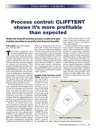
Process control: CLIFFTENT
shows it’s more profitable
than expected
Model the tradeoff between process credits and spec
violation penalties to quantify total financial benefits
Specs
CV targets
Operator
limits
Process operating region
Optimum setting of CV targets
Fig. 1. Optimum CV targets may exceed specification.

2. Profitability of CMVPC is primar-
ily determined by properly setting CV
limits. If they are set too tight, nar-
row, and conservative and constrain
the controller, it becomes almost
inactive and generates little value.
If they are set too loose, wide, liberal
and open beyond the valid domain of
the model, improper bouncing into
dangerous or unstable regions gener-
ates losses. CV limits must be set by
people “just right.” This is central to
the art of CMVPC.
CVs are also dependent variables
in LP/SQP models. These models are
built to predict CVs from MVs and
independent measured and unmea-
sured disturbance variables (DVs).
The optimizing algorithms select the
best (optimum) values for MV and cor-
responding CV5, 6. For LP formula-
tions, we know the solution will lie at
an intersection of CV limits and MV
constraints in n-space for n-MV. LP is
a corner picker in n-space (Fig. 1). The
art of LP planning goes beyond getting
model slopes right, it is critical to set
dependent variable CV limits right.
LPs do not set CV limits, people do.
Set them too tight and profit improve-
ment is invariably small; set them too
wide and model validity vanishes, the
solution is not physically feasible and
profit improvement again vanishes.
Profitability of a planning LP model
solution is primarily determined by
properly setting dependent variable
CV limit values.
While nonlinear SQP may find
an interior top of a hill optima, it is
invariably partially (highly partially)
constrained at a partial hill corner in
n-space because
o p t i m u m H P I
plant operation is
at a combination
of CV and MV con-
straints and equip-
ment limits. SQP is
a corner-hill picker.
The art of CLRTO
goes beyond getting
the process model
for capacity, yield
and operating costs
right. It is critical
to set dependent
variable CV limits
right.
The profitabil-
ity of an opera-
tor, manager or a
plant is primar-
ily determined by
properly setting operating CV limits.
If set too tight with large safety mar-
gins and big quality giveaways, yields
suffer, operating costs are excessive
and capacity is curtailed so the plant
is inefficient and uneconomic. If set
too loose with inadequate safety mar-
gins and excessive quality violations,
the plant becomes unreliable, unsafe
and uneconomic. If we push process
credits for yield, operating costs and
capacity too far against equipment
and quality specs, the risk of severe
consequences always rises. One of
plant management’s basic jobs is reg-
ular assessment of the proper tradeoff
between safe operating margins and
technical competitiveness. CV limits
must be set properly.
These decisions are basic tradeoffs
of knowledge and risk. They lie at the
heart of decisions between the oper-
ating and technical departments in
every HPI plant.7
This article describes for the first
time the method for properly setting
CV high and low limit values (targets
for the mean) in the neighborhood of
specs set by people to maximize profit.
It introduces the concept of CLIFF-
TENT, the key function required to
determine CV limits and dynamic
performance value. It illustrates the
essential role of modeling the penalty
for violating the spec; modeling the
consequences of breaking the rules,
to properly set CV limits.
Almost all decisions involve recon-
ciling a tradeoff between a “process”
credit and a less tangible risk of pen-
alty if we “break the rules.” The proper
car speed target (cruise control set-
ting) is a tradeoff between the value
of a shorter trip against the chance
and penalty of citation or accident. We
model both types of dissimilar phenom-
ena and reconcile them to find the best
(optimum) speed target. For those with
little incentive for a short trip and high
uncertainty and penalty of citation,
it is best to “play it on the safe side”
and their optimum speed target is
below the posted limit. For those with
large incentive for a shorter trip and
low uncertainty and penalty of cita-
tion, their optimum speed target may
exceed the posted limit. Indianapolis
racers and marathon runners face a
similar tradeoff; we all do.
For CMVPC and CLRTO (and
human operators for that matter) to
work well, the computer (or opera-
tor) must know how the plant works
(the process model), what the plant
operating purpose is (the financial
objective function), what the rules
are (specs or CV limits) and what the
financial consequences will be for
breaking the rules (CV penalties).
Without all of these, they will not
work well.
These problems all come together
with CLIFFTENT. It provides the
rigorous modeling framework to con-
nect these issues and solve them. The
CLIFFTENT method needs two input
functions: frequency distribution and
unit profit. It finds a third function:
time profit.
Traditional justification. CVs vary
in time. A base case illustrated in Fig.
2 shows a CV transient varying about
its mean, below its upper limit spec.
CLIFFTENT can be illustrated with
a simple example: manufacturing an
average 10 Mbpd of low sulfur fuel
oil (LSFO). Fig. 2 plots LSFO sulfur
content for shipments over the past T
= six months. The quality spec is xs =
1.0 w%S max, the mean is miu = 0.9
w%S and standard deviation is sd =
0.06 w%S.
Traditional process control benefits
are assessed by estimating control per-
formance improvement and assuming it
first provides a degree of reduced fluc-
tuations about the same mean shown
in Fig. 2 (say sd = 0.02). Most assume
this base case mean is OK, optimal at
the start (we will show this is invari-
ably incorrect). They then assume this
smoother operation provides no tan-
gible benefit itself (because they do not
know how to quantify it), but take this
as a necessary prerequisite to the sec-
76 HYDROCARBON PROCESSING / DECEMBER 1996
Fig. 2. Traditional justification method.

3. ond step, move the mean an appropri-
ate amount closer to the spec (“appro-
priate” is arbitrary because they do
not know how to properly set the new
mean either), so say 0.05 to 0.095. Then
they multiply the CV mean change by
some flow/CV factor to get improved
yield, capacity or utility consumption
(say 5,000 bpd cutter /%S). This is in
turn multiplied by a $/day per unit flow
factor (say $2.5/bbl cutter) to estimate
$/day profit gain (625). The missing
ingredient is failure to model the pen-
alty for violating the spec limit.1
Frequency distribution function.
The frequency distribution function,
f(x), provides the number of units of
material at each value, x, of a CV of
interest as a function of x. It is the sta-
tistical distribution of CV data with
mean, miu, and standard deviation,
sd, over a time period, T. This func-
tion must be provided or assumed; it
is an input requirement. It is taken
directly from the transient data. It
may be Normal Gaussian or arbitrary,
provided it is bounded, integrable and
its integral is also bounded. Most use-
ful, of course, is if we can assume it to
be stationary for some period until a
new f(x) can be determined.
The sulfur content distribution for
our example LSFO shipments over
the past six months is the second
curve shown in Fig. 3.
Unit profit function. The unit profit
function, UP(x), provides the profit
per unit (bbl, lb, ton, cargo) of mate-
rial (usually feed or a product) at
each value, x, of a CV of interest as a
function of x.1 This function must be
provided or assumed; it is an input
requirement. It must become negative
in both directions, for very small x and
for very large x. It may have disconti-
nuities and be arbitrary provided it is
bounded, integrable and its integral is
also bounded. Most useful, of course,
is if we can assume it to be stationary
for some period until a new UP(x) can
be determined.
For the LSFO example, if prod-
uct is precisely and consistently just
within spec xs = 1.0 w%S, profit is
$1.00/bbl LSFO, from the function
plot at the top of Fig. 3. Our steady-
state process model for cutter stock
blending and hydrodesulfurization
shows unit profit declines if sulfur
is below spec, x < xs, and product is too
pure, because operating costs increase:
excessive valuable cutter, H2 and cata-
lyst, and lower yield/higher feed. The
profit decline for quality giveaway to
the left below spec may be nonlinear,
and curvature is usually downward.
In theory, UP(x) may increase at first
below spec for interior CV optima (if
product price increases faster than
costs increase, for example), but this
rarely occurs for product quality. If x
is low enough, unit profit vanishes,
UP(x) < 0, and product manufacture
is in the red. The LSFO example in
Table 1 is shown in Fig. 4.
The sales contract for most of this
example LSFO is to a utility boiler
with a $0.6/bbl penalty cliff if a cargo
exceeds spec xs = 1.00, plus an increas-
ing penalty proportional to the size of
the violation because the utility must
blend valuable cutter into the boiler
or pay an SO2 permit noncompliance
fine. The profit decline to the right
above the spec may be nonlinear, and
curvature is usually downward. In
theory, UP (x) may increase at first
above spec for interior CV optima,
but these are very rare. If x is high
enough, unit profit vanishes, UP(x)
< 0, and product manufacture is in
the red.
The LHS below spec, UP(x), x <
xs, is the process performance model;
the slope in an LP matrix for profit
against this CV, LSFO sulfur con-
tent. The RHS above spec, UP(x), x
> xs, is the customer dissatisfaction
model. The unit profit function gives
the magnitude and range (tent) of CV
profitability. It is highly nonlinear at
the spec; it usually has discontinu-
ous slope and value. It describes the
financial effects people associate with
the value, x, of the CV. People must
ultimately determine this CLIFF-
TENT function, UP(x). It is a model-
ing activity beyond LP, SQP, CLRTO,
and CMVPC.
In fact, we have answered a com-
mon, previously unanswered ques-
tion of process control and LP mod-
eling: how does one identify CV
dependent variables? How do we
recognize one when we see it? How
do we select among the enormous
number of possible candidate CVs?
Are all T, P, L, comp-i at every point
in all processes to become a CV? Why
not? Our opening definition of CV
provides the answer. Each CV has a
UP(x), a CLIFFTENT of consequence.
If a variable has or can be assigned
a CLIFFTENT it is a CV, if not it is
not. A CV is not what we can model
or measure; that comes later. A CV
is first a variable we know, we care
about, we value, it matters and we
can assign it a CLIFFTENT. Then
if UP(x) is interesting, large, signifi-
HYDROCARBON PROCESSING / DECEMBER 1996 77
Fig. 3. The second curve shows the sulfur content distribution.
Fig. 4. Graphic representation of LSFO example in Table 1.

4. cant or crucial we go about measur-
ing and modeling it, then controlling
and optimizing it. That is the essence
of plant operation.
Time profit. In view of Figs. 3 and 4,
is the CV distribution mean, miu = 0.9
(at fixed sd = 0.06) properly aligned
with UP(x)? Is miu = 0.9 optimal or
should it be higher or lower, and by
how much? Raise it closer to spec xs =
1.00, but not all the way. How much
money would be generated by setting
it right, optimally, in the first place?
Integrating f(x) and UP(x) pro-
vides the time profit, TP (miu = 0.9) =
$6,488.9 /d average for T = 6 months.
We find the entire function TP (miu,
0.06) shown in the middle of Figs. 3
and 4. It is a hill; it has a maximum of
$6,805.7/d at optimum miu = 0.933 for
a profit gain of $316.8/d, (Table 1).
This CLIFFTENT integral is the
rigorous method for setting the tar-
get mean of a CV close to its spec. It
accounts for statistical uncertainty
and dynamic performance, sd, pro-
cess performance model, spec viola-
tion penalty and profit at spec. The
optimum CV target may even exceed
spec when the pro-
cess incentive slope
is steep and spec
violation penalty
is shallow. This is
shown in the lower
part of Fig. 1.
C L I F F T E N T
provides the rig-
orous modeling
method for taking
calculated risks on
the right hand side
(RHS) and quan-
tifying the intan-
gibles. It shows
clearly where the
money comes from;
less low profit prod-
uct at the far left
hand side (LHS) and far RHS.
We see the true time profit func-
tion near the optimum mean target
is a smoother hill, even if UP(x) has a
discontinuity. The true profit function
with uncertainty at CV limits and LP
constraints in Fig. 1 is really not so
sharp as a line or cliff, it is a rounder
“donut.” The slope of the profit func-
tion at LP constraints is really zero,
not the “shadow price.” This is why LP
“shadow prices” are so unrealistic and
useless in practice. The CLIFFTENT
modeling concept transcends LP and
SQP optimization technology.
A multivariable controller (MVC)
needs CV weighting factors to dis-
tinguish the relative ranking impor-
tance among all its CVs, with dissim-
ilar engineering units and scaling,
to account for differences in their
interest and importance. When the
number of CVs exceeds the number
of MVs and degrees of freedom, some
CVs cannot be controlled at limits;
they must remain inside. One MVC
calls the weighting factors “equal
concern errors” (ECE), representing
the amount of each CV limit viola-
tion that represents equivalent pen-
alty, say $100/d loss. The MVC for
a fluid catalytic cracking unit has
more than 50 CVs for equipment lim-
its and product qualities; each CV
needs an “equal concern error.” The
TP(miu) penalty side provides this
parameter also. This controller also
needs profit values for its imbedded
LP. The TP(miu) credit side provides
this information.
Comparing profits. CLIFFTENT
provides the rigorous method to com-
pare profits if any of the input param-
eters change. It quantifies the new
proper CV limit and corresponding
profit change. These can come from
changes in process performance
(LHS), customer market or contract
(CLIFF penalty), corporate efficiency
(UP(xs)) or dynamic performance, sd.
These are listed in Table 1.
For example, suppose improved
analysis and control of LSFO sulfur
content from the refinery HDS and
blender reduces sd from 0.06 to 0.02.
The new TP(miu, 0.02), the fourth
curve in Figs. 3 and 5, shows TP(0.933,
0.02) = 7,938.3 – TP(0.933, 0.06) =
6,805.7, which provides $1,132.6/d
more profit from reduced variance
alone about the same original opti-
mum mean of 0.933. Then, if the mean
is increased to its new optimum 0.965,
TP(0.965, 0.02) = 8,672.1, which gives
an additional profit of $733.8/d. The
hidden previously intangible benefit
from improved dynamic performance
and reduced variance about the origi-
nal optimum mean is 1,132.6/1,866.4
= 60.7% of the total benefit achievable.
The optimally located distribution is
the bottom in Figs. 3 and 5.
Where does this value come from?
It comes from less spec violations and
less quality cost giveaway. This is
shown in Fig. 5. These can never be
quantified unless the violation pen-
alty is modeled first.
If UP(x) is linear over the range
of the distribution, f(x), we can prove
reducing sd provides no profit increase;
credits from one side equal debits from
the other side. That is why tighter
accumulator level control makes no
money unless it reduces the frequency
of overflow or drainage mishaps. Cur-
vature and discontinuity nonlinear-
ity in the UP(x) function provides the
incentive for improving dynamic per-
formance and smoother operation. The
greater the nonlinearity, the greater
the incentive. The total CLIFFTENT
concept is illustrated in Fig. 5.
78 HYDROCARBON PROCESSING / DECEMBER 1996
Table 1. LSFO example
Problem:
Spec xs = 1.0 w%S, max. Capacity = 10 Mbpd
UP (xs) = $1.0/bbl Left curvature = −1
Cliff = $−0.6/bbl Right curvature = −0.8
Left slope = $5/bbl/%S Normal dist. mean = 0.90 w%S
Right slope = $−3/bbl/%S Normal dist. sd = 0.06 w%S
Solution: Comparison: sd = 0.02 w%S
Opt. mean = 0.933 w%S Opt. mean = 0.965 w%S
TP (0.9, 0.06) = $6,488.9/d TP (0.933, 0.02) = $7,938.3/d
TP (0.9267, 0.06) = $6,805.7/d Del.TPdynmcs = $1,132.6/d
Del.TPstdystate = $316.8/d TP (0.965, 0.02) = $8,672.1/d
Del.TPstdystate = $733.8/d
Del.TPtotl = $1,866.4/d
Fig. 5 The bottom curve is the optimally located distribution.

5. Connection to RE. CLIFFTENT pro-
vides the rigorous modeling method to
connect process models for conservation
mass momentum and energy balances,
for yield, operating cost and capacity
performance to the surrounding world
of RE (Table 2): customers, safety, main-
tenance, environment, human values,
and money balance. RE stands for so
many of these activities like recheck,
refund, replace, recycle, reprocess, etc.,
listed in Table 2. It provides the finan-
cial connecting link between operating
condition target setting and risk man-
agement like HAZOPS. It provides the
connection between statistical process/
quality control, and dynamic process
control. It provides the connection
between CLRTO and CMVPC. It pro-
vides the connection between quality
and value.
CLIFFTENT connects oil indus-
try process modeling methods to the
modeling methods of an equally large
industry: insurance. Modeling meth-
ods in the land of RE often require
techniques of statistics, expected
values, life expectancy, cost of occur-
rence and risk management central
to the insurance industry. In light of
CLIFFTENT, many would agree that
the fuels and chemicals industries
may have overemphasized (easier?)
modeling the chemistry and physics of
processes and neglected modeling the
world of RE: economic and business
issues. Now, with CLIFFTENT, we
know how to use these two dissimi-
lar modeling approaches to estimate
profit improvement.
Examples. Several additional exam-
ples of tradeoffs that have been mod-
eled, solved and optimized in oil refin-
ing illustrate the breadth of generality
and usefulness of the CLIFFTENT
method.
Atomospheric crude unit. Atmo-
spheric crude distillation tower side
draw kerosine (KE) is more valu-
able than overhead naphtha (NA) in
Japan and many other regions. The
key quality spec is kerosine minimum
(IBP) and (FP) to recover valuable KE
lost in the overhead NA. The penalties
for off-spec KE include nonoptimum
blending and low top tray tempera-
ture, dew point, liquid phase acid and
corrosion.
Vacuum unit. Raising vacuum
unit furnace temperature increases
recovery of valuable VGO for FCC
feed from black VRESID. The penal-
ties are increased furnace tube cok-
ing, metal fatigue and metals in VGO
which contaminate FCC catalyst.
FCC compressor. Raising reac-
tor and wet gas compressor suction
pressure releases compressor horse-
power capacity for increased feed or
conversion. The penalties are more
frequent relief spills of lost gas to flare
and negative environmental impact
and community relations.
FCC slide valve. Reducing FCC
regenerated catalyst slide valve dif-
ferential pressure (DP) releases air
blower and wet gas compressor capac-
ity and operating costs worth about
$1 million/yr/psi for a large 100 Mbpd
FCC. The penalties of very low DP are
increased frequency of cat circulation
reversal, oil feed to the regenerator,
catalyst damage and lost products
costing 0.2 to 1.0 MM$/occurrence.
Gasoline octane. Lowering gaso-
line octane increases reformate yield
and process efficiency, which increases
profit/bbl gasoline. The penalties if
octane is too low are customer com-
plaints from engine knock and reduc-
tion in market volume and/or price.
Delayed coker. Reducing delayed
coker drum fill outage increases its
capacity to process feed. The penalties
are increased frequency of foam over
to the main fractionator and expen-
sive cleanouts.
High loads cause distillation flood-
HYDROCARBON PROCESSING / DECEMBER 1996 79
Table 2. Spec violation modeling: the world of “RE”
Breech Hazop Reprocess
Cancellation Injury Reprimand
Carryover1 Insurance Reputation
Cavitation2 Inventory Rerun
Citation Late penalty Resample
Coking Litigation Reship
Complaints Losses Resubmit
Corrosion Overpressure Return
Damages Plugging Reversal6
Deactivation Reblend Revise
Default Recall Rework
Demurrage Recheck Risk manage-
ment
Discount Recycle Safety
Discharge Redo Scrap
Downgrade Reflux Settlement
Explosion Refund Spill
Fatigue3 Reject Stream factor
Fine Relief5 Surge7
Fire Repair Turndown
Flaring Repeal Turnover
Flooding4 Repeat Venting
Fouling Replace Violation8
1 Entrainment, foaming
2 Pump
3 Tube metal temperature
4 Distillation
5 Valves
6 FCC catalyst circulation
7 Compressor
8 Permit, regulation, law
Table 3. Conclusions: to increase profit
1. Optimize miu, mean target Know your business and product
Make best use of what you have
Set targets right
2. Decrease sigma, variance Maintain smooth control
Lower variance alone makes
money
3. Increase UPm Raise sell price
Cut fixed costs
4. Decrease m1, positive slope Raise process efficiency
Lower variable costs
5. Increase m2, negative slope Improve customer good will
Lower complaints
6. Decrease CLIFF Obey the law
Plan for emergencies
7. Increase C, capacity Expand markets
Raise production rate
8. Increase max. xs or Negotiate for looser spec
decrease min. xs Reassess basis for spec
9. If Tpmax (optmean) < 0, Sell out fast
no matter what Liquidate
Table 4. CLIFFTENT results - base
Situation analysis
1. Time profit, function of CV mean
2. Max. time profit
3. Optimize CV target
4. Profit increase = max. − base
5. Controller variable ranking, ECE
6. Amount of unprofitable product, %
7. % of perfect control profit

6. ing, compressor stall and vibration,
separator liquid entrainment carryover,
packed bed channeling, pump cavita-
tion, reactors to loose conversion or
depart from equilibrium, heater huffing
and pipe vibration. Low loads cause dis-
tillation weeping, compressor surge and
heater flame outs. Each piece of equip-
ment has a maximum capacity indica-
tor and minimum turndown capacity
indicator. These phenomena in the
world of RE can be modeled financially
to create the CLIFFTENT to set targets
optimally. The reader should be able to
readily identify the modeling work for
a particular process situation.
Reducing unforseen conse-
quences. There is a lot of money to
be made by setting CV targets in the
HPI right. One large U.S. oil refiner
(1 MMbpd) recently reported concern
about “$60 million/yr in unforeseen
occurrences in 1995.” The troubling
word is “unforeseen.” Modeling CLIFF-
TENT penalties and setting CV limits
for maximum expected profit would
significantly reduce the “unforeseen.”
Deploying CMVPC and CLRTO would
significantly reduce the 60. Quantify-
ing all the options in Table 3 provides
a comprehensive approach to assessing
business profitability improvements.
In fact, CLIFFTENT provides the
mechanism for reconciling more gen-
eral conflicts and tradeoffs. Everyday
risks like cancer from smoking (1 in
3), death from traffic (1 in 5,000),
workplace injury (1 in 5,000), death as
a pedestrian (1 in 40,000) and cancer
from living near nuclear reactors (1 in
100,000,000) might be better quanti-
fied by CLIFFTENT analysis because
Harvard’s Public Health Dept. stud-
ies8 show “we may be spending enor-
mous amounts of money on problems
that may pose trivial risk. Under-
standing risk comes down to under-
standing the difference between the
product of very small probabilities
times high penalties—that requires
analysis, not intu-
ition, because peo-
ple have very poor conception of how
to think of very small probabilities.”
Witness the Lotto and Las Vegas.
Public policy issues that affect the
HPI like clean fuel composition, envi-
ronmental emissions and safe opera-
tions need scientifically based cost/ben-
efit analysis with careful modeling of
human values to optimize the tradeoffs
and reduce or resolve conflicts. This
might even be the method for properly
setting interest rate, growth, inflation
and unemployment CV targets.
Results from CLIFFTENT analy-
ses (Tables 4 and 5), confirm that pre-
viously intangible benefits of dynamic
process control are of the same order
of magnitude as simplified estimates
of tangible benefits,1 so the true merit
is about double that normally (con-
servatively) claimed. What has been
invisible now becomes visible. What
has been suspected can now be proven.
Table 6 summarizes conclusions from
the CLIFFTENT approach.
Many (perhaps most?) process con-
trol and information system projects
are launched using the “faith theory”:
computers are good; everybody is doing
it; surely we can cut fuel 3%, improve
yield 1%, increase capacity 2% and
that is plenty of money; and modern
technology is inherently wonderful.
Before embarking with the “faith the-
ory” alone, the CLIFFTENT approach
validates what the Greeks taught in
400 BC: Do analysis before synthesis,
function comes before form. The pre-
requisites are: 1) know your process
and, how it works; 2) know your objec-
tive and purpose; 3) know the rules
and limits; 4) know the consequences
and penalties for breaking the rules
and violating the limits, and 5) deploy
CLIFFTENT analysis to bring your
knowledge together, to set CV targets
properly and to optimize profit. If you
first know what you are going to do,
why you plan to do it and how you will
measure success and failure, then it
becomes much easier to figure out how
to do it; how to harness computers to
do a good job improving profits.
LITERATURE CITED
1 Latour, P. R., “Quantify quality control’s intangible
benefits,” Hydrocarbon Processing, Vol. 71, No. 5, May
1992, p. 61.
2 Latour, P. R., “APC & RIS,” FUEL, Mar/Apr 1992, Vol. 2,
No. 2, p. 14.
3 Latour, P. R., “Plan to use RIS/APC for Manufacturing
RFG/LSD,” FUEL, Jul/Aug 1994, Vol. 4, No. 4., p. 20
4 HPI Market Data Book, Hydrocarbon Processing, 1993.
5 Latour, P. R., “Online computer optimization 1: What it is
and where to do it,” Hydrocarbon Processing, June 1979,
Vol. 58, No. 6, p. 73.
6 Latour, P. R., “Online computer optimization 2: benefits
and implementation,” Hydrocarbon Processing, July
1979, Vol. 58, No. 7, p. 219.
7 Anderson, R. F., “Total cost of ownership: getting past
the 10% solution,” Hydrocarbon Processing, Vol. 75, No.
7, July 1996, p. 105.
8 Vedantam, Shankar, “High anxiety over low risks,”
Houston Chronicle, April 5, 1996, p. 8A.
80 HYDROCARBON PROCESSING / DECEMBER 1996
Table 5. CLIFFTENT results - comparison
Improve dynamic performance
1. New time profit, function of CV mean
2. Dynamic profit = TP (μ1
0 σ2) − TP (μ1
0 σ1)
3. New max. time profit = TP (μ2
0 σ2)
4. New opt. CV target = μ2
0
5. Steady state profit = TP (μ2
0 σ2) − TP (μ1
0 σ2)
6. Total Δ profit = DYN + SS = TP (μ2
0 σ2) − TP (μ1
0 σ1)
7. New controller variable ranking, ECE
8. New amount of unprofitable product, %
9. New % of perfect control profit
Table 6. CLIFFTENT summary
Given: distribution and CLIFFTENT functions
1. Can specify value of CV target to maximize expected
profit
2. Can quantify financial benefit from improved dynamic per-
formance, reduced variance, smoother CV operation
3. Can connect SQC SPC/APC, MVC/RTO, process model/
surroundings impact, risk/profit
4. Can convert intangibles/experience/human judgment into
analytical knowledge modeling for calculated risk taking, to
maximize expected profit from dissimilar phenomena
5. Can optimize any tradeoff with uncertainty
6. Can connect oil industry and computer industry with insur-
ance industry
7. Can minimize unforeseen occurences
The author
Pierre R. Latour has
been vice president of
Aspen Technology, Inc.
since it acquired DMCC
and Setpoint in Jan. ’96.
Dr. Latour is implement-
ing DMC controllers on
FCCs and ACUs in the
U.S. and Japan, develop-
ing performance-based technology licensing,
managing third-party relations and develop-
ing strategic cimfuels business. He joined
DMCC as vice president in June ’95 after
taking early retirement from Setpoint in
Feb. ’95.
Dr. Latour cofounded Setpoint in 1977 and
served as a director and vice president of
consulting, oil refining, central marketing
and business development. He founded Set-
point Japan in ’84 and served as chairman,
BOD, for 11 years. He began his career with
DuPont and Shell Oil, inaugurating computer
control of the Deer Park, Texas FCC in ’66.
After two years as captain, U.S. Army at
NASA Manned Spacecraft Center manag-
ing the Apollo docking simulator program,
he cofounded Biles & Associates, Inc. Dr.
Latour has worked on contracts for 50 HPI
companies around the world. He special-
izes in identifying, capturing and sustaining
benefits from process computer control. He
earned a BS degree in chemical engineering
from Virginia Tech and PhD degree in chemi-
cal engineering from Purdue. He is cimfuels
editor for FUEL and a registered PE in Texas
and California.