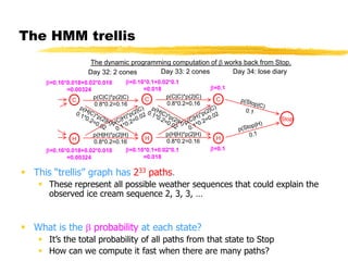
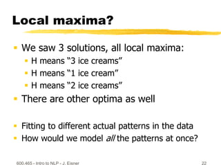
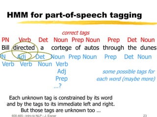
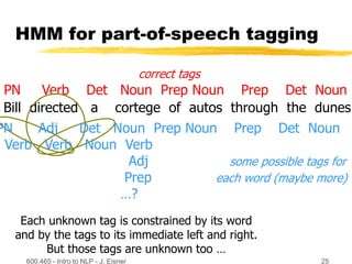
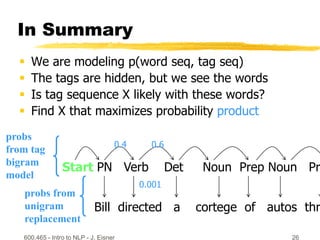
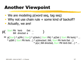
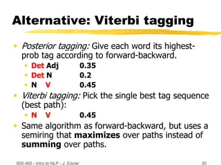
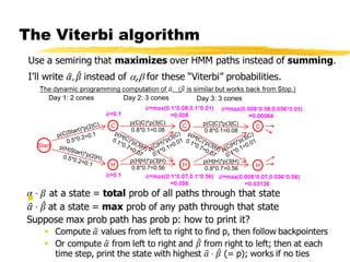
600.465 - Intro to NLP - J. Eisner 1
Hidden Markov Models
and the Forward-Backward
Algorithm
600.465 - Intro to NLP - J. Eisner 2
Please See the Spreadsheet
 I like to teach this material using an
interactive spreadsheet:
 http://cs.jhu.edu/~jason/papers/#tnlp02
 Has the spreadsheet and the lesson plan
 I’ll also show the following slides at
appropriate points.
600.465 - Intro to NLP - J. Eisner 3
Marginalization
SALES Jan Feb Mar Apr …
Widgets 5 0 3 2 …
Grommets 7 3 10 8 …
Gadgets 0 0 1 0 …
… … … … … …
600.465 - Intro to NLP - J. Eisner 4
Marginalization
SALES Jan Feb Mar Apr … TOTAL
Widgets 5 0 3 2 … 30
Grommets 7 3 10 8 … 80
Gadgets 0 0 1 0 … 2
… … … … … …
TOTAL 99 25 126 90 1000
Write the totals in the margins
Grand total
600.465 - Intro to NLP - J. Eisner 5
Marginalization
prob. Jan Feb Mar Apr … TOTAL
Widgets .005 0 .003 .002 … .030
Grommets .007 .003 .010 .008 … .080
Gadgets 0 0 .001 0 … .002
… … … … … …
TOTAL .099 .025 .126 .090 1.000
Grand total
Given a random sale, what & when was it?
600.465 - Intro to NLP - J. Eisner 6
Marginalization
prob. Jan Feb Mar Apr … TOTAL
Widgets .005 0 .003 .002 … .030
Grommets .007 .003 .010 .008 … .080
Gadgets 0 0 .001 0 … .002
… … … … … …
TOTAL .099 .025 .126 .090 1.000
Given a random sale, what & when was it?
marginal prob: p(Jan)
marginal
prob:
p(widget)
joint prob: p(Jan,widget)
marginal prob:
p(anything in table)
600.465 - Intro to NLP - J. Eisner 7
Conditionalization
prob. Jan Feb Mar Apr … TOTAL
Widgets .005 0 .003 .002 … .030
Grommets .007 .003 .010 .008 … .080
Gadgets 0 0 .001 0 … .002
… … … … … …
TOTAL .099 .025 .126 .090 1.000
Given a random sale in Jan., what was it?
marginal prob: p(Jan)
joint prob: p(Jan,widget)
conditional prob: p(widget|Jan)=.005/.099
p(… | Jan)
.005/.099
.007/.099
0
…
.099/.099
Divide column
through by Z=0.99
so it sums to 1
600.465 - Intro to NLP - J. Eisner 8
Marginalization & conditionalization
in the weather example
 Instead of a 2-dimensional table,
now we have a 66-dimensional table:
 33 of the dimensions have 2 choices: {C,H}
 33 of the dimensions have 3 choices: {1,2,3}
 Cross-section showing just 3 of the dimensions:
Weather2=C Weather2=H
IceCream2=1 0.000… 0.000…
IceCream2=2 0.000… 0.000…
IceCream2=3 0.000… 0.000…
600.465 - Intro to NLP - J. Eisner 9
Interesting probabilities in
the weather example
 Prior probability of weather:
p(Weather=CHH…)
 Posterior probability of weather (after observing evidence):
p(Weather=CHH… | IceCream=233…)
 Posterior marginal probability that day 3 is hot:
p(Weather3=H | IceCream=233…)
= w such that w3=H p(Weather=w | IceCream=233…)
 Posterior conditional probability
that day 3 is hot if day 2 is:
p(Weather3=H | Weather2=H, IceCream=233…)
600.465 - Intro to NLP - J. Eisner 10
The HMM trellis
Day 1: 2 cones
Start
C
H
C
H
Day 2: 3 cones
C
H
p(H|H)*p(3|H)
0.8*0.7=0.56
p(H|H)*p(3|H)
0.8*0.7=0.56
Day 3: 3 cones
 This “trellis” graph has 233 paths.
 These represent all possible weather sequences that could explain the
observed ice cream sequence 2, 3, 3, …
p(C|C)*p(3|C)
0.8*0.1=0.08
p(C|C)*p(3|C)
0.8*0.1=0.08
C C
H
p(C|C)*p(3|C)
p(C|C)*p(2|C)
p(C|C)*p(1|C)
The trellis represents only such
explanations. It omits arcs that were
a priori possible but inconsistent with
the observed data. So the trellis arcs
leaving a state add up to < 1.
600.465 - Intro to NLP - J. Eisner 11
The HMM trellis
The dynamic programming computation of a works forward from Start.
Day 1: 2 cones
Start
C
H
C
H
Day 2: 3 cones
C
H
p(H|H)*p(3|H)
0.8*0.7=0.56
p(H|H)*p(3|H)
0.8*0.7=0.56
Day 3: 3 cones
 This “trellis” graph has 233 paths.
 These represent all possible weather sequences that could explain the
observed ice cream sequence 2, 3, 3, …
 What is the product of all the edge weights on one path H, H, H, …?
 Edge weights are chosen to get p(weather=H,H,H,… & icecream=2,3,3,…)
 What is the a probability at each state?
 It’s the total probability of all paths from Start to that state.
 How can we compute it fast when there are many paths?
a=0.1*0.07+0.1*0.56
=0.063
a=0.1*0.08+0.1*0.01
=0.009
a=0.1
a=0.1 a=0.009*0.07+0.063*0.56
=0.03591
a=0.009*0.08+0.063*0.01
=0.00135
a=1
p(C|C)*p(3|C)
0.8*0.1=0.08
p(C|C)*p(3|C)
0.8*0.1=0.08
600.465 - Intro to NLP - J. Eisner 12
Computing a Values
C
H
p2
f
d
e
All paths to state:
a = (ap1 + bp1 + cp1)
+ (dp2 + ep2 + fp2)
= a1p1 + a2p2
a2
C
p1
a
b
c
a1
a
Thanks, distributive law!
 This “trellis” graph has 233 paths.
 These represent all possible weather sequences that could explain the
observed ice cream sequence 2, 3, 3, …
600.465 - Intro to NLP - J. Eisner 13
The HMM trellis
Day 34: lose diary
Stop
C
H
p(C|C)*p(2|C)
0.8*0.2=0.16
p(H|H)*p(2|H)
0.8*0.2=0.16
b=0.16*0.1+0.02*0.1
=0.018
b=0.16*0.1+0.02*0.1
=0.018
Day 33: 2 cones
b=0.1
C
H
p(C|C)*p(2|C)
0.8*0.2=0.16
p(H|H)*p(2|H)
0.8*0.2=0.16
b=0.16*0.018+0.02*0.018
=0.00324
b=0.16*0.018+0.02*0.018
=0.00324
Day 32: 2 cones
The dynamic programming computation of b works back from Stop.
 What is the b probability at each state?
 It’s the total probability of all paths from that state to Stop
 How can we compute it fast when there are many paths?
C
H
b=0.1
600.465 - Intro to NLP - J. Eisner 14
Computing b Values
C
H
p2
z
x
y
All paths from state:
b = (p1u + p1v + p1w)
+ (p2x + p2y + p2z)
= p1b1 + p2b2
C
p1
u
v
w
b2
b1
b
600.465 - Intro to NLP - J. Eisner 15
Computing State Probabilities
C
x
y
z
a
b
c
All paths through state:
ax + ay + az
+ bx + by + bz
+ cx + cy + cz
= (a+b+c)(x+y+z)
= a(C)  b(C)
a b
Thanks, distributive law!
600.465 - Intro to NLP - J. Eisner 16
Computing Arc Probabilities
C
H
p
x
y
z
a
b
c
All paths through the p arc:
apx + apy + apz
+ bpx + bpy + bpz
+ cpx + cpy + cpz
= (a+b+c)p(x+y+z)
= a(H)  p  b(C)
a
b
Thanks, distributive law!
Maximizing (Log-)Likelihood

600.465 - Intro to NLP - J. Eisner 17
Local maxima?
 We saw 3 solutions, all local maxima:
600.465 - Intro to NLP - J. Eisner 18
600.465 - Intro to NLP - J. Eisner 19
600.465 - Intro to NLP - J. Eisner 20
600.465 - Intro to NLP - J. Eisner 21
Local maxima?
 We saw 3 solutions, all local maxima:
 H means “3 ice creams”
 H means “1 ice cream”
 H means “2 ice creams”
 There are other optima as well
 Fitting to different actual patterns in the data
 How would we model all the patterns at once?
600.465 - Intro to NLP - J. Eisner 22
600.465 - Intro to NLP - J. Eisner 23
HMM for part-of-speech tagging
Bill directed a cortege of autos through the dunes
PN Verb Det Noun Prep Noun Prep Det Noun
correct tags
Each unknown tag is constrained by its word
and by the tags to its immediate left and right.
But those tags are unknown too …
PN Adj Det Noun Prep Noun Prep Det Noun
Verb Verb Noun Verb
Adj some possible tags for
Prep each word (maybe more)
…?
600.465 - Intro to NLP - J. Eisner 24
Bill directed a cortege of autos through the dunes
PN Verb Det Noun Prep Noun Prep Det Noun
correct tags
Each unknown tag is constrained by its word
and by the tags to its immediate left and right.
But those tags are unknown too …
HMM for part-of-speech tagging
PN Adj Det Noun Prep Noun Prep Det Noun
Verb Verb Noun Verb
Adj some possible tags for
Prep each word (maybe more)
…?
600.465 - Intro to NLP - J. Eisner 25
Bill directed a cortege of autos through the dunes
PN Verb Det Noun Prep Noun Prep Det Noun
correct tags
Each unknown tag is constrained by its word
and by the tags to its immediate left and right.
But those tags are unknown too …
HMM for part-of-speech tagging
PN Adj Det Noun Prep Noun Prep Det Noun
Verb Verb Noun Verb
Adj some possible tags for
Prep each word (maybe more)
…?
600.465 - Intro to NLP - J. Eisner 26
In Summary
 We are modeling p(word seq, tag seq)
 The tags are hidden, but we see the words
 Is tag sequence X likely with these words?
 Find X that maximizes probability product
Start PN Verb Det Noun Prep Noun Pr
Bill directed a cortege of autos thr
0.4 0.6
0.001
probs
from tag
bigram
model
probs from
unigram
replacement
600.465 - Intro to NLP - J. Eisner 27
Another Viewpoint
 We are modeling p(word seq, tag seq)
 Why not use chain rule + some kind of backoff?
 Actually, we are!
Start PN Verb Det …
Bill directed a …
p( )
= p(Start) * p(PN | Start) * p(Verb | Start PN) * p(Det | Start PN Verb) * …
* p(Bill | Start PN Verb …) * p(directed | Bill, Start PN Verb Det …)
* p(a | Bill directed, Start PN Verb Det …) * …
600.465 - Intro to NLP - J. Eisner 28
Another Viewpoint
 We are modeling p(word seq, tag seq)
 Why not use chain rule + some kind of backoff?
 Actually, we are!
Start PN Verb Det …
Bill directed a …
p( )
= p(Start) * p(PN | Start) * p(Verb | Start PN) * p(Det | Start PN Verb) * …
* p(Bill | Start PN Verb …) * p(directed | Bill, Start PN Verb Det …)
* p(a | Bill directed, Start PN Verb Det …) * …
Start PN Verb Det Noun Prep Noun Prep Det Noun Stop
Bill directed a cortege of autos through the dunes
600.465 - Intro to NLP - J. Eisner 29
Posterior tagging
 Give each word its highest-prob tag according to
forward-backward.
 Do this independently of other words.
 Det Adj 0.35
 Det N 0.2
 N V 0.45
 Output is
 Det V 0
 Defensible: maximizes expected # of correct tags.
 But not a coherent sequence. May screw up
subsequent processing (e.g., can’t find any parse).
 exp # correct tags = 0.55+0.35 = 0.9
 exp # correct tags = 0.55+0.2 = 0.75
 exp # correct tags = 0.45+0.45 = 0.9
 exp # correct tags = 0.55+0.45 = 1.0
600.465 - Intro to NLP - J. Eisner 30
Alternative: Viterbi tagging
 Posterior tagging: Give each word its highest-
prob tag according to forward-backward.
 Det Adj 0.35
 Det N 0.2
 N V 0.45
 Viterbi tagging: Pick the single best tag sequence
(best path):
 N V 0.45
 Same algorithm as forward-backward, but uses a
semiring that maximizes over paths instead of
summing over paths.
600.465 - Intro to NLP - J. Eisner 31
The Viterbi algorithm
Day 1: 2 cones
Start
C
H
C
H
p(C|C)*p(3|C)
0.8*0.1=0.08
p(H|H)*p(3|H)
0.8*0.7=0.56
Day 2: 3 cones
C
H
p(C|C)*p(3|C)
0.8*0.1=0.08
p(H|H)*p(3|H)
0.8*0.7=0.56
Day 3: 3 cones


Hidden Markov Model in Natural Language Processing

  • 1.
    600.465 - Introto NLP - J. Eisner 1 Hidden Markov Models and the Forward-Backward Algorithm
  • 2.
    600.465 - Introto NLP - J. Eisner 2 Please See the Spreadsheet  I like to teach this material using an interactive spreadsheet:  http://cs.jhu.edu/~jason/papers/#tnlp02  Has the spreadsheet and the lesson plan  I’ll also show the following slides at appropriate points.
  • 3.
    600.465 - Introto NLP - J. Eisner 3 Marginalization SALES Jan Feb Mar Apr … Widgets 5 0 3 2 … Grommets 7 3 10 8 … Gadgets 0 0 1 0 … … … … … … …
  • 4.
    600.465 - Introto NLP - J. Eisner 4 Marginalization SALES Jan Feb Mar Apr … TOTAL Widgets 5 0 3 2 … 30 Grommets 7 3 10 8 … 80 Gadgets 0 0 1 0 … 2 … … … … … … TOTAL 99 25 126 90 1000 Write the totals in the margins Grand total
  • 5.
    600.465 - Introto NLP - J. Eisner 5 Marginalization prob. Jan Feb Mar Apr … TOTAL Widgets .005 0 .003 .002 … .030 Grommets .007 .003 .010 .008 … .080 Gadgets 0 0 .001 0 … .002 … … … … … … TOTAL .099 .025 .126 .090 1.000 Grand total Given a random sale, what & when was it?
  • 6.
    600.465 - Introto NLP - J. Eisner 6 Marginalization prob. Jan Feb Mar Apr … TOTAL Widgets .005 0 .003 .002 … .030 Grommets .007 .003 .010 .008 … .080 Gadgets 0 0 .001 0 … .002 … … … … … … TOTAL .099 .025 .126 .090 1.000 Given a random sale, what & when was it? marginal prob: p(Jan) marginal prob: p(widget) joint prob: p(Jan,widget) marginal prob: p(anything in table)
  • 7.
    600.465 - Introto NLP - J. Eisner 7 Conditionalization prob. Jan Feb Mar Apr … TOTAL Widgets .005 0 .003 .002 … .030 Grommets .007 .003 .010 .008 … .080 Gadgets 0 0 .001 0 … .002 … … … … … … TOTAL .099 .025 .126 .090 1.000 Given a random sale in Jan., what was it? marginal prob: p(Jan) joint prob: p(Jan,widget) conditional prob: p(widget|Jan)=.005/.099 p(… | Jan) .005/.099 .007/.099 0 … .099/.099 Divide column through by Z=0.99 so it sums to 1
  • 8.
    600.465 - Introto NLP - J. Eisner 8 Marginalization & conditionalization in the weather example  Instead of a 2-dimensional table, now we have a 66-dimensional table:  33 of the dimensions have 2 choices: {C,H}  33 of the dimensions have 3 choices: {1,2,3}  Cross-section showing just 3 of the dimensions: Weather2=C Weather2=H IceCream2=1 0.000… 0.000… IceCream2=2 0.000… 0.000… IceCream2=3 0.000… 0.000…
  • 9.
    600.465 - Introto NLP - J. Eisner 9 Interesting probabilities in the weather example  Prior probability of weather: p(Weather=CHH…)  Posterior probability of weather (after observing evidence): p(Weather=CHH… | IceCream=233…)  Posterior marginal probability that day 3 is hot: p(Weather3=H | IceCream=233…) = w such that w3=H p(Weather=w | IceCream=233…)  Posterior conditional probability that day 3 is hot if day 2 is: p(Weather3=H | Weather2=H, IceCream=233…)
  • 10.
    600.465 - Introto NLP - J. Eisner 10 The HMM trellis Day 1: 2 cones Start C H C H Day 2: 3 cones C H p(H|H)*p(3|H) 0.8*0.7=0.56 p(H|H)*p(3|H) 0.8*0.7=0.56 Day 3: 3 cones  This “trellis” graph has 233 paths.  These represent all possible weather sequences that could explain the observed ice cream sequence 2, 3, 3, … p(C|C)*p(3|C) 0.8*0.1=0.08 p(C|C)*p(3|C) 0.8*0.1=0.08 C C H p(C|C)*p(3|C) p(C|C)*p(2|C) p(C|C)*p(1|C) The trellis represents only such explanations. It omits arcs that were a priori possible but inconsistent with the observed data. So the trellis arcs leaving a state add up to < 1.
  • 11.
    600.465 - Introto NLP - J. Eisner 11 The HMM trellis The dynamic programming computation of a works forward from Start. Day 1: 2 cones Start C H C H Day 2: 3 cones C H p(H|H)*p(3|H) 0.8*0.7=0.56 p(H|H)*p(3|H) 0.8*0.7=0.56 Day 3: 3 cones  This “trellis” graph has 233 paths.  These represent all possible weather sequences that could explain the observed ice cream sequence 2, 3, 3, …  What is the product of all the edge weights on one path H, H, H, …?  Edge weights are chosen to get p(weather=H,H,H,… & icecream=2,3,3,…)  What is the a probability at each state?  It’s the total probability of all paths from Start to that state.  How can we compute it fast when there are many paths? a=0.1*0.07+0.1*0.56 =0.063 a=0.1*0.08+0.1*0.01 =0.009 a=0.1 a=0.1 a=0.009*0.07+0.063*0.56 =0.03591 a=0.009*0.08+0.063*0.01 =0.00135 a=1 p(C|C)*p(3|C) 0.8*0.1=0.08 p(C|C)*p(3|C) 0.8*0.1=0.08
  • 12.
    600.465 - Introto NLP - J. Eisner 12 Computing a Values C H p2 f d e All paths to state: a = (ap1 + bp1 + cp1) + (dp2 + ep2 + fp2) = a1p1 + a2p2 a2 C p1 a b c a1 a Thanks, distributive law!
  • 13.
     This “trellis”graph has 233 paths.  These represent all possible weather sequences that could explain the observed ice cream sequence 2, 3, 3, … 600.465 - Intro to NLP - J. Eisner 13 The HMM trellis Day 34: lose diary Stop C H p(C|C)*p(2|C) 0.8*0.2=0.16 p(H|H)*p(2|H) 0.8*0.2=0.16 b=0.16*0.1+0.02*0.1 =0.018 b=0.16*0.1+0.02*0.1 =0.018 Day 33: 2 cones b=0.1 C H p(C|C)*p(2|C) 0.8*0.2=0.16 p(H|H)*p(2|H) 0.8*0.2=0.16 b=0.16*0.018+0.02*0.018 =0.00324 b=0.16*0.018+0.02*0.018 =0.00324 Day 32: 2 cones The dynamic programming computation of b works back from Stop.  What is the b probability at each state?  It’s the total probability of all paths from that state to Stop  How can we compute it fast when there are many paths? C H b=0.1
  • 14.
    600.465 - Introto NLP - J. Eisner 14 Computing b Values C H p2 z x y All paths from state: b = (p1u + p1v + p1w) + (p2x + p2y + p2z) = p1b1 + p2b2 C p1 u v w b2 b1 b
  • 15.
    600.465 - Introto NLP - J. Eisner 15 Computing State Probabilities C x y z a b c All paths through state: ax + ay + az + bx + by + bz + cx + cy + cz = (a+b+c)(x+y+z) = a(C)  b(C) a b Thanks, distributive law!
  • 16.
    600.465 - Introto NLP - J. Eisner 16 Computing Arc Probabilities C H p x y z a b c All paths through the p arc: apx + apy + apz + bpx + bpy + bpz + cpx + cpy + cpz = (a+b+c)p(x+y+z) = a(H)  p  b(C) a b Thanks, distributive law!
  • 17.
    Maximizing (Log-)Likelihood  600.465 -Intro to NLP - J. Eisner 17
  • 18.
    Local maxima?  Wesaw 3 solutions, all local maxima: 600.465 - Intro to NLP - J. Eisner 18
  • 19.
    600.465 - Introto NLP - J. Eisner 19
  • 20.
    600.465 - Introto NLP - J. Eisner 20
  • 21.
    600.465 - Introto NLP - J. Eisner 21
  • 22.
    Local maxima?  Wesaw 3 solutions, all local maxima:  H means “3 ice creams”  H means “1 ice cream”  H means “2 ice creams”  There are other optima as well  Fitting to different actual patterns in the data  How would we model all the patterns at once? 600.465 - Intro to NLP - J. Eisner 22
  • 23.
    600.465 - Introto NLP - J. Eisner 23 HMM for part-of-speech tagging Bill directed a cortege of autos through the dunes PN Verb Det Noun Prep Noun Prep Det Noun correct tags Each unknown tag is constrained by its word and by the tags to its immediate left and right. But those tags are unknown too … PN Adj Det Noun Prep Noun Prep Det Noun Verb Verb Noun Verb Adj some possible tags for Prep each word (maybe more) …?
  • 24.
    600.465 - Introto NLP - J. Eisner 24 Bill directed a cortege of autos through the dunes PN Verb Det Noun Prep Noun Prep Det Noun correct tags Each unknown tag is constrained by its word and by the tags to its immediate left and right. But those tags are unknown too … HMM for part-of-speech tagging PN Adj Det Noun Prep Noun Prep Det Noun Verb Verb Noun Verb Adj some possible tags for Prep each word (maybe more) …?
  • 25.
    600.465 - Introto NLP - J. Eisner 25 Bill directed a cortege of autos through the dunes PN Verb Det Noun Prep Noun Prep Det Noun correct tags Each unknown tag is constrained by its word and by the tags to its immediate left and right. But those tags are unknown too … HMM for part-of-speech tagging PN Adj Det Noun Prep Noun Prep Det Noun Verb Verb Noun Verb Adj some possible tags for Prep each word (maybe more) …?
  • 26.
    600.465 - Introto NLP - J. Eisner 26 In Summary  We are modeling p(word seq, tag seq)  The tags are hidden, but we see the words  Is tag sequence X likely with these words?  Find X that maximizes probability product Start PN Verb Det Noun Prep Noun Pr Bill directed a cortege of autos thr 0.4 0.6 0.001 probs from tag bigram model probs from unigram replacement
  • 27.
    600.465 - Introto NLP - J. Eisner 27 Another Viewpoint  We are modeling p(word seq, tag seq)  Why not use chain rule + some kind of backoff?  Actually, we are! Start PN Verb Det … Bill directed a … p( ) = p(Start) * p(PN | Start) * p(Verb | Start PN) * p(Det | Start PN Verb) * … * p(Bill | Start PN Verb …) * p(directed | Bill, Start PN Verb Det …) * p(a | Bill directed, Start PN Verb Det …) * …
  • 28.
    600.465 - Introto NLP - J. Eisner 28 Another Viewpoint  We are modeling p(word seq, tag seq)  Why not use chain rule + some kind of backoff?  Actually, we are! Start PN Verb Det … Bill directed a … p( ) = p(Start) * p(PN | Start) * p(Verb | Start PN) * p(Det | Start PN Verb) * … * p(Bill | Start PN Verb …) * p(directed | Bill, Start PN Verb Det …) * p(a | Bill directed, Start PN Verb Det …) * … Start PN Verb Det Noun Prep Noun Prep Det Noun Stop Bill directed a cortege of autos through the dunes
  • 29.
    600.465 - Introto NLP - J. Eisner 29 600.465 - Intro to NLP - J. Eisner 29 Posterior tagging  Give each word its highest-prob tag according to forward-backward.  Do this independently of other words.  Det Adj 0.35  Det N 0.2  N V 0.45  Output is  Det V 0  Defensible: maximizes expected # of correct tags.  But not a coherent sequence. May screw up subsequent processing (e.g., can’t find any parse).  exp # correct tags = 0.55+0.35 = 0.9  exp # correct tags = 0.55+0.2 = 0.75  exp # correct tags = 0.45+0.45 = 0.9  exp # correct tags = 0.55+0.45 = 1.0
  • 30.
    600.465 - Introto NLP - J. Eisner 30 600.465 - Intro to NLP - J. Eisner 30 Alternative: Viterbi tagging  Posterior tagging: Give each word its highest- prob tag according to forward-backward.  Det Adj 0.35  Det N 0.2  N V 0.45  Viterbi tagging: Pick the single best tag sequence (best path):  N V 0.45  Same algorithm as forward-backward, but uses a semiring that maximizes over paths instead of summing over paths.
  • 31.
    600.465 - Introto NLP - J. Eisner 31 The Viterbi algorithm Day 1: 2 cones Start C H C H p(C|C)*p(3|C) 0.8*0.1=0.08 p(H|H)*p(3|H) 0.8*0.7=0.56 Day 2: 3 cones C H p(C|C)*p(3|C) 0.8*0.1=0.08 p(H|H)*p(3|H) 0.8*0.7=0.56 Day 3: 3 cones 