It is about general and basics about Thermodynamics

1. Lectures on Heat and Thermodynamics
Physics 152
Michael Fowler, University of Virginia 8/30/08
Contents
HEAT...........................................................................................................................................................3
Feeling and seeing temperature changes.....................................................................................3
Classic Dramatic Uses of Temperature-Dependent Effects..........................................................4
The First Thermometer........................................................................................................................5
Newton’s Anonymous Table of Temperatures ...............................................................................7
Fahrenheit’s Excellent Thermometer ...............................................................................................7
Amontons’ Air Thermometer: Pressure Increases Linearly with Temperature .............................7
Thermal Equilibrium and the Zeroth Law of Thermodynamics......................................................8
Measuring Heat Flow: a Unit of Heat...............................................................................................8
Specific Heats and Calorimetry .......................................................................................................9
A Connection With Atomic Theory ................................................................................................10
Latent Heat.......................................................................................................................................11
THERMAL EXPANSION AND THE GAS LAW.............................................................................................12
Coefficients of Expansion................................................................................................................12
Gas Pressure Increase with Temperature......................................................................................13
Finding a Natural Temperature Scale............................................................................................13
The Gas Law .....................................................................................................................................14
Avogadro’s Hypothesis....................................................................................................................15
EARLY ATTEMPTS TO UNDERSTAND THE NATURE OF HEAT .....................................................................16
When Heat Flows, What, Exactly is Flowing? ................................................................................16
Lavoisier’s Caloric Fluid Theory .......................................................................................................16
The Industrial Revolution and the Water Wheel ...........................................................................17
Measuring Power by Lifting.............................................................................................................18
Carnot’s Caloric Water Wheel .......................................................................................................18
How Efficient are these Machines? ...............................................................................................19
Count Rumford.................................................................................................................................20
Rumford’s Theory of Heat................................................................................................................22
THE DISCOVERY OF ENERGY CONSERVATION: MAYER AND JOULE ....................................................24
Robert Mayer and the Color of Blood...........................................................................................24
James Joule......................................................................................................................................26
But Who Was First: Mayer or Joule? ...............................................................................................27
The Emergence of Energy Conservation ......................................................................................27
KINETIC THEORY OF GASES: A BRIEF REVIEW.........................................................................................28

2. 2
Bernoulli's Picture..............................................................................................................................28
The Link between Molecular Energy and Pressure ......................................................................29
Maxwell finds the Velocity Distribution ..........................................................................................30
Velocity Space.................................................................................................................................31
Maxwell’s Symmetry Argument......................................................................................................32
What about Potential Energy?.......................................................................................................37
Degrees of Freedom and Equipartition of Energy .......................................................................39
Brownian Motion ..............................................................................................................................39
IDEAL GAS THERMODYNAMICS: SPECIFIC HEATS, ISOTHERMS, ADIABATS..........................................39
Introduction: the Ideal Gas Model, Heat, Work and Thermodynamics....................................39
The Gas Specific Heats CV and CP.................................................................................................40
Tracking a Gas in the (P, V) Plane: Isotherms and Adiabats ......................................................42
Equation for an Adiabat .................................................................................................................44
HEAT ENGINES: THE CARNOT CYCLE .....................................................................................................46
The Ultimate in Fuel Efficiency ........................................................................................................46
Step 1: Isothermal Expansion ..........................................................................................................47
Step 2: Adiabatic Expansion...........................................................................................................48
Steps 3 and 4: Completing the Cycle ...........................................................................................49
Efficiency of the Carnot Engine .....................................................................................................51
THE LAWS OF THERMODYNAMICS AND LIMITS ON ENGINE EFFICIENCY.............................................53
The Laws of Thermodynamics.........................................................................................................53
How the Second Law Limits Engine Efficiency .............................................................................55
A NEW THERMODYNAMIC VARIABLE: ENTROPY ...................................................................................57
Introduction ......................................................................................................................................57
Heat Changes along Different Paths from a to c are Different! ................................................57
But Something Heat Related is the Same: Introducing Entropy.................................................59
Finding the Entropy Difference for an Ideal Gas..........................................................................61
Entropy in Irreversible Change: Heat Flow Without Work............................................................62
Entropy Change without Heat Flow: Opening a Divided Box....................................................62
The Third Law of Thermodynamics.................................................................................................64
ENTROPY AND THE KINETIC THEORY: THE MOLECULAR PICTURE ..........................................................64
Searching for a Molecular Description of Entropy.......................................................................64
Enter the Demon ..............................................................................................................................65
Boltzmann Makes the Breakthrough..............................................................................................66
Epitaph: S = k ln W............................................................................................................................68
But What Are the Units for Measuring W ? ....................................................................................68
A More Dynamic Picture.................................................................................................................68
The Removed Partition: What Are the Chances of the Gas Going Back?...............................69
Demon Fluctuations.........................................................................................................................70
Entropy and “Disorder”....................................................................................................................71
Summary: Entropy, Irreversibility and the Meaning of Never......................................................71
Everyday Examples of Irreversible Processes ................................................................................72
MOLECULAR COLLISIONS.......................................................................................................................73
Difficulties Getting the Kinetic Theory Moving..............................................................................73
How Fast Are Smelly Molecules?....................................................................................................73
The Mean Free Path.........................................................................................................................74

3. 3
Gas Viscosity Doesn’t Depend on Density!...................................................................................74
Gas Diffusion: the Pinball Scenario; Finding the Mean Free Path in Terms of the Molecular
Diameter ...........................................................................................................................................74
But the Pinball Picture is Too Simple: the Target Molecules Are Moving!..................................78
If Gases Intermingle 0.5cm in One Second, How Far in One Hour? ..........................................78
Actually Measuring Mean Free Paths............................................................................................79
Why did Newton get the Speed of Sound Wrong?.....................................................................80
BROWNIAN MOTION...............................................................................................................................80
Introduction: Jiggling Pollen Granules...........................................................................................80
Einstein’s Theory: the Osmosis Analogy .........................................................................................81
An Atmosphere of Yellow Spheres.................................................................................................83
Langevin’s Theory ............................................................................................................................84
References........................................................................................................................................86
HEAT TRANSPORT: CONDUCTION, CONVECTION, RADIATION ............................................................87
Conduction.......................................................................................................................................87
Microscopic Picture of Conduction...............................................................................................87
American Units..................................................................................................................................88
Convection.......................................................................................................................................88
Radiation...........................................................................................................................................89
Heat
Feeling and seeing temperature changes
Within some reasonable temperature range, we can get a rough idea how warm something is by
touching it. But this can be unreliable—if you put one hand in cold water, one in hot, then plunge
both of them into lukewarm water, one hand will tell you it’s hot, the other will feel cold. For
something too hot to touch, we can often get an impression of how hot it is by approaching and
sensing the radiant heat. If the temperature increases enough, it begins to glow and we can see it’s
hot!
The problem with these subjective perceptions of heat is that they may not be the same for
everybody. If our two hands can’t agree on whether water is warm or cold, how likely is it that a
group of people can set a uniform standard? We need to construct a device of some kind that
responds to temperature in a simple, measurable way—we need a thermometer.
The first step on the road to a thermometer was taken by one Philo of Byzantium, an engineer, in the
second century BC. He took a hollow lead sphere connected with a tight seal to one end of a pipe,
the other end of the pipe being under water in another vessel.

4. 4
To quote Philo: “…if you expose the sphere to the sun, part of the air enclosed in the tube will pass
out when the sphere becomes hot. This will be evident because the air will descend from the tube
into the water, agitating it and producing a succession of bubbles.
Now if the sphere is put back in the shade, that is, where the sun’s rays do not reach it, the water
will rise and pass through the tube …”
“No matter how many times you repeat the operation, the same thing will happen.
In fact, if you heat the sphere with fire, or even if you pour hot water over it, the result will be the
same.”
Notice that Philo did what a real investigative scientist should do—he checked that the experiment
was reproducible, and he established that the air’s expansion was in response to heat being applied
to the sphere, and was independent of the source of the heat.
Classic Dramatic Uses of Temperature-Dependent Effects
This expansion of air on heating became widely known in classical times, and was used in
various dramatic devices. For example, Hero of Alexandria describes a small temple where a
fire on the altar causes the doors to open.

5. 5
The altar is a large airtight box, with a pipe leading from it to another enclosed container filled with
water. When the fire is set on top of the altar, the air in the box heats up and expands into a second
container which is filled with water. This water is forced out through an overflow pipe into a bucket
hung on a rope attached to the door hinges in such a way that as the bucket fills with water, it drops,
turns the hinges, and opens the doors. The pipe into this bucket reaches almost to the bottom, so
that when the altar fire goes out, the water is sucked back and the doors close again. (Presumably,
once the fire is burning, the god behind the doors is ready to do business and the doors open…)
Still, none of these ingenious devices is a thermometer. There was no attempt (at least none
recorded) by Philo or his followers to make a quantitative measurement of how hot or cold the
sphere was. And the “meter” in thermometer means measurement.
The First Thermometer
Galileo claimed to have invented the first thermometer. Well, actually, he called it a thermoscope,
but he did try to measure “degrees of heat and cold” according to a colleague, and that qualifies it as
a thermometer. (Technically, a thermoscope is a device making it possible to see a temperature
change, a thermometer can measure the temperature change.) Galileo used an inverted narrow-
necked bulb with a tubular neck, like a hen’s egg with a long glass tube attached at the tip.

6. 6
He first heated the bulb with his hands then immediately put it into water. He recorded that the
water rose in the bulb the height of “one palm”. Later, either Galileo or his colleague Santorio
Santorio put a paper scale next to the tube to read off changes in the water level. This definitely
made it a thermometer, but who thought of it first isn’t clear (they argued about it). And, in fact,
this thermometer had problems.
Question: what problems? If you occasionally top up the water, why shouldn’t this thermometer be
good for recording daily changes in temperature?
Answer: because it’s also a barometer! But—Galileo didn’t know about the atmospheric pressure.
Torricelli, one of Galileo’s pupils, was the first to realize, shortly after Galileo died, that the real
driving force in suction was external atmospheric pressure, a satisfying mechanical explanation in
contrast to the philosophical “nature abhors a vacuum”. In the 1640’s, Pascal pointed out that the
variability of atmospheric pressure rendered the air thermometer untrustworthy.
Liquid-in-glass thermometers were used from the 1630’s, and they were of course insensitive to
barometric pressure. Meteorological records were kept from this time, but there was no real
uniformity of temperature measurement until Fahrenheit, almost a hundred years later.

7. 7
Newton’s Anonymous Table of Temperatures
The first systematic account of a range of different temperatures, “Degrees of Heat”, was written by
Newton, but published anonymously, in 1701. Presumably he felt that this project lacked the
timeless significance of some of his other achievements.
Taking the freezing point of water as zero, Newton found the temperature of boiling water to be
almost three times that of the human body, melting lead eight times as great (actually 327C,
whereas 8x37=296, so this is pretty good!) but for higher temperatures, such as that of a wood fire,
he underestimated considerably. He used a linseed oil liquid in glass thermometer up to the melting
point of tin (232°C). (Linseed oil doesn’t boil until 343°C, but that is also its autoignition
temperature!)
Newton tried to estimate the higher temperatures indirectly. He heated up a piece of iron in a fire,
then let it cool in a steady breeze. He found that, at least at the lower temperatures where he could
cross check with his thermometer, the temperature dropped in a geometric progression, that is, if it
took five minutes to drop from 80° above air temperature to 40° above air temperature, it took
another five minutes to drop to 20° above air, another five to drop to 10° above, and so on. He then
assumed this same pattern of temperature drop was true at the high temperatures beyond the reach
of his thermometer, and so estimated the temperature of the fire and of iron glowing red hot. This
wasn’t very accurate—he (under)estimated the temperature of the fire to be about 600°C.
Fahrenheit’s Excellent Thermometer
The first really good thermometer, using mercury expanding from a bulb into a capillary tube, was
made by Fahrenheit in the early 1720’s. He got the idea of using mercury from a colleague’s
comment that one should correct a barometer reading to allow for the variation of the density of
mercury with temperature. The point that has to be borne in mind in constructing thermometers,
and defining temperature scales, is that not all liquids expand at uniform rates on heating—water,
for example, at first contracts on heating from its freezing point, then begins to expand at around
forty degrees Fahrenheit, so a water thermometer wouldn’t be very helpful on a cold day. It is also
not easy to manufacture a uniform cross section capillary tube, but Fahrenheit managed to do it, and
demonstrated his success by showing his thermometers agreed with each other over a whole range
of temperatures. Fortunately, it turns out that mercury is well behaved in that the temperature scale
defined by taking its expansion to be uniform coincides very closely with the true temperature scale,
as we shall see later.
Amontons’ Air Thermometer: Pressure Increases Linearly with
Temperature
A little earlier (1702) Amontons introduced an air pressure thermometer. He established that if air
at atmospheric pressure (he states 30 inches of mercury) at the freezing point of water is enclosed
then heated to the boiling point of water, but meanwhile kept at constant volume by increasing the

8. 8
pressure on it, the pressure goes up by about 10 inches of mercury. He also discovered that if he
compressed the air in the first place, so that it was at a pressure of sixty inches of mercury at the
temperature of melting ice, then if he raised its temperature to that of boiling water, at the same time
adding mercury to the column to keep the volume of air constant, the pressure increased by 20
inches of mercury. In other words, he found that for a fixed amount of air kept in a container at
constant volume, the pressure increased with temperature by about 33% from freezing to boiling,
that percentage being independent of the initial pressure.
Thermal Equilibrium and the Zeroth Law of Thermodynamics
Once the thermometer came to be widely used, more precise observations of temperature and (as we
shall see) heat flow became possible. Joseph Black, a professor at the University of Edinburgh in the
1700’s, noticed that a collection of objects at different temperatures, if brought together, will all
eventually reach the same temperature.
As he wrote, “By the use of these instruments [thermometers] we have learned, that if we take 1000,
or more, different kinds of matter, such as metals, stones, salts, woods, cork, feathers, wool, water
and a variety of other fluids, although they be all at first of different heats, let them be placed
together in a room without a fire, and into which the sun does not shine, the heat will be
communicated from the hotter of these bodies to the colder, during some hours, perhaps, or the
course of a day, at the end of which time, if we apply a thermometer to all of them in succession, it
will point to precisely the same degree.”
We say nowadays that bodies in “thermal contact” eventually come into “thermal equilibrium”—
which means they finally attain the same temperature, after which no further heat flow takes place.
This is equivalent to:
The Zeroth Law of Thermodynamics:
If two objects are in thermal equilibrium with a third, then they are in thermal equilibrium
with each other.
The “third body” in a practical situation is just the thermometer.
It’s perhaps worth pointing out that this trivial sounding statement certainly wasn’t obvious before
the invention of the thermometer. With only the sense of touch to go on, few people would agree
that a piece of wool and a bar of metal, both at 0°C, were at the same temperature.
Measuring Heat Flow: a Unit of Heat
The next obvious question is, can we get more quantitative about this “flow of heat” that takes place
between bodies as they move towards thermal equilibrium? For example, suppose I reproduce one

9. 9
of Fahrenheit’s experiments, by taking 100 ccs of water at 100°F, and 100ccs at 150°F, and mix
them together in an insulated jug so little heat escapes. What is the final temperature of the mix?
Of course, it’s close to 125°F—not surprising, but it does tell us something! It tells us that the
amount of heat required to raise the temperature of 100 cc of water from 100°F to 125°F is exactly
the same as the amount needed to raise it from 125°F to 150°F. A series of such experiments (done
by Fahrenheit, Black and others) established that it always took the same amount of heat to raise the
temperature of 1 cc of water by one degree.
This makes it possible to define a unit of heat. Perhaps unfairly to Fahrenheit,
1 calorie is the heat required to raise the temperature of 1 gram of water by 1 degree
Celsius.
(Celsius also lived in the early 1700’s. His scale has the freezing point of water as 0°C, the boiling
point as 100°C. Fahrenheit’s scale is no longer used in science, but lives on in engineering in the
US, and in the British Thermal Unit, which is the heat required to raise the temperature of one
pound of water by 1°F.)
Specific Heats and Calorimetry
First, let’s define specific heat:
The specific heat of a substance is the heat required in calories to raise the temperature of
1 gram by 1 degree Celsius.
As Fahrenheit continues his measurements of heat flow, it quickly became evident that for
different materials, the amount of heat needed to raise the temperature of one gram by one
degree could be quite different. For example, it had been widely thought before the
measurements were made, that one cc of Mercury, being a lot heavier than one cc of water,
would take more heat to raise its temperature by one degree. This proved not to be the case—
Fahrenheit himself made the measurement. In an insulating container, called a “calorimeter” he
added 100ccs of water at 100°F to 100ccs of mercury at 150°F, and stirred so they quickly
reached thermal equilibrium.
Question: what do you think the final temperature was? Approximately?
Answer: The final temperature was, surprisingly, about 120°F. 100 cc of water evidently
“contained more heat” than 100 cc of mercury, despite the large difference in weight!

10. 10
This technique, called calorimetry, was widely used to find the specific heats of many different
substances, and at first no clear pattern emerged. It was puzzling that the specific heat of mercury
was so low compared with water! As more experiments on different substances were done, it
gradually became evident that heavier substances, paradoxically, had lower specific heats.
A Connection With Atomic Theory
Meanwhile, this quantitative approach to scientific observation had spread to chemistry. Towards
the end of the 1700’s, Lavoisier weighed chemicals involved in reactions before and after the
reaction. This involved weighing the gases involved, so had to be carried out in closed containers,
so that, for example, the weight of oxygen used and the carbon dioxide, etc., produced would
accounted for in studying combustion. The big discovery was that mass was neither created nor
destroyed. This had not been realized before because no one had weighed the gases involved. It
made the atomic theory suddenly more plausible, with the idea that maybe chemical reactions were
just rearrangements of atoms into different combinations.
Lavoisier also clarified the concept of an element, an idea that was taken up in about 1800 by John
Dalton, who argues that a given compound consisted of identical molecules, made up of elementary
atoms in the same proportion, such as H2O (although that was thought initially to be HO). This
explained why, when substances reacted chemically, such as the burning of hydrogen to form water,
it took exactly eight grams of oxygen for each gram of hydrogen. (Well, you could also produce
H2O2 under the right conditions, with exactly sixteen grams of oxygen to one of hydrogen, but the
simple ratios of amounts of oxygen needed for the two reactions were simply explained by different
molecular structures, and made the atomic hypothesis even more plausible.)
Much effort was expended carefully weighing the constituents in many chemical reactions, and
constructing diagrams of the molecules. The important result of all this work was that it became
possible to list the relative weights of the atoms involved. For example, the data on H2O and H2O2
led to the conclusion that an oxygen atom weighed sixteen times the weight of a hydrogen atom.
It must be emphasized, though, that these results gave no clue as to the actual weights of atoms! All
that was known was that atoms were too small to see in the best microscopes. Nevertheless,
knowing the relative weights of some atoms in 1820 led to an important discovery. Two professors
in France, Dulong and Petit, found that for a whole series of elements the product of atomic weight
and specific heat was the same!

11. 11
Element Specific Heat Relative weights of
the atoms
Product of relative
atomic weight and
specific heat
Lead 0.0293 12.95 0.3794
Tin 0.0514 7.35 0.3779
Zinc 0.0927 4.03 0.3736
Sulphur 0.1880 2.011 0.3780
The significance of this, as they pointed out, was that the “specific heat”, or heat capacity, of
each atom was the same—a piece of lead and a piece of zinc having the same number of atoms
would have the same heat capacity. So heavier atoms absorbed no more heat than lighter atoms
for a given rise in temperature. This partially explained why mercury had such a surprisingly
low heat capacity. Of course, having no idea how big the atoms might be, they could go no
further. And, indeed, many of their colleagues didn’t believe in atoms anyway, so it was hard to
convince them of the significance of this discovery.
Latent Heat
One of Black’s experiments was to set a pan of water on a steady fire and observe the temperature
as a function of time. He found it steadily increased, reflecting the supply of heat from the fire, until
the water began to boil, whereupon the temperature stayed the same for a long time. The steam
coming off was at the same (boiling) temperature as the water. So what was happening to the heat
being supplied? Black correctly concluded that heat needed to be supplied to change water from its
liquid state to its gaseous state, that is, to steam. In fact, a lot of heat had to be supplied: 540
calories per gram, as opposed to the mere 100 calories per gram needed to bring it from the freezing
temperature to boiling. He also discovered that it took 80 calories per gram to melt ice into water,
with no rise in temperature. This heat is released when the water freezes back to ice, so it is
somehow “hidden” in the water. He called it latent heat, meaning hidden heat.
__________________________________________________________________________
Books I used in preparing this lecture:
A Source Book in Greek Science, M. R. Cohen and I. E. Drabkin, Harvard university Press, 1966.
A History of the Thermometer and its Uses in Meteorology, W. E. Knowles Middleton, Johns
Hopkins Press, 1966.
A Source Book in Physics, W. F. Magie, McGraw-Hill, New York, 1935.

12. 12
Thermal Expansion and the Gas Law
Coefficients of Expansion
Almost all materials expand on heating—the most famous exception being water, which
contracts as it is warmed from 0 degrees Celsius to 4 degrees. This is actually a good thing,
because as freezing weather sets in, the coldest water, which is about to freeze, is less dense than
slightly warmer water, so rises to the top of a lake and the ice begins to form there. For almost
all other liquids, solidification on cooling begins at the bottom of the container. So, since water
behaves in this weird way, ice skating is possible! Also, as a matter of fact, life in lakes is
possible—the ice layer that forms insulates the rest of the lake water from very cold air, so fish
can make it through the winter.
Linear Expansion
The coefficient of linear expansion α of a given material, for example a bar of copper, at a given
temperature is defined as the fractional increase in length that takes place on heating through one
degree:
( ) 0
1 when 1L L L L T Tα→ + Δ = + → + C
Of course, α might vary with temperature (it does for water, as we just mentioned) but in fact
for most materials it stays close to constant over wide temperature ranges.
For copper, 6
17 10 .α −
= ×
Volume Expansion
For liquids and gases, the natural measure of expansion is the coefficient of volume
expansion, β .
( ) 0
1 when 1V V V V T Tβ→ + Δ = + → + C
Of course, on heating a bar of copper, clearly the volume as well as the length increases—the bar
expands by an equal fraction in all directions (this could be experimentally verified, or you could
just imagine a cube of copper, in which case all directions look the same).
The volume of a cube of copper of side L is V = L3
. Suppose we heat it through one degree.
Putting together the definitions of ,α β above,
( ) ( ) ( ) ( )
3 33 3
1 , 1 , 1 or 1V V L L L L Vβ α α→ + → + → + → + .Vα

13. 13
So ( ) (
3
1 1 )β α+ = + . But remember α is very, very small—so even though
( )
3 2
1 1 3 3 3
α α α α+ = + + + , the last two terms are completely negligible (check it out!) so to a
fantastically good approximation:
3 .β α=
The coefficient of volume expansion is just three times the coefficient of linear expansion.
Gas Pressure Increase with Temperature
In 1702, Amontons discovered a linear increase of P with T for air, and found P to increase
about 33% from the freezing point of water to the boiling point of water.
That is to say, he discovered that if a container of air were to be sealed at 0°C, at ordinary
atmospheric pressure of 15 pounds per square inch, and then heated to 100°C but kept at the
same volume, the air would now exert a pressure of about 20 pounds per square inch on the sides
of the container. (Of course, strictly speaking, the container will also have increased in size, that
would lower the effect—but it’s a tiny correction, about ½% for copper, even less for steel and
glass.)
Remarkably, Amontons discovered, if the gas were initially at a pressure of thirty pounds per
square inch at 0°C, on heating to 100°C the pressure would go to about 40 pounds per square
inch—so the percentage increase in pressure was the same for any initial pressure: on heating
through 100°C, the pressure would always increase by about 33%.
Furthermore, the result turned out to be the same for different gases!
Finding a Natural Temperature Scale
In class, we plotted air pressure as a function of temperature for a fixed volume of air, by making
several measurements as the air was slowly heated (to give it a chance to all be at the same
temperature at each stage). We found a straight line. On the graph, we extended the line
backwards, to see how the pressure would presumably drop on cooling the air. We found the
remarkable prediction that the pressure should drop to zero at a temperature of about −273°C.
In fact, if we’d done the cooling experiment, we would have found that air doesn’t actually
follow the line all the way down, but condenses to a liquid at around −200°C. However, helium
gas stays a gas almost to −270°C, and follows the line closely.

14. 14
We shall discuss the physics of gases, and the interpretation of this, much more fully in a couple
of lectures. For now, the important point is that this suggests a much more natural temperature
scale than the Celsius one: we should take −273°C as the zero of temperature! For one thing, if
we do that, the pressure/temperature relationship for a gas becomes beautifully simple:
.P T∝
This temperature scale, in which the degrees have the same size as in Celsius, is called the
Kelvin or absolute scale. Temperatures are written 300K. To get from Celsius to Kelvin, just
add 273 (strictly speaking, 273.15).
An Ideal Gas
Physicists at this point introduce the concept of an “Ideal Gas”. This is like the idea of a
frictionless surface: it doesn’t exist in nature, but it is a very handy approximation to some real
systems, and makes problems much easier to handle mathematically. The ideal gas is one for
which for all temperatures, so helium is close to ideal over a very wide range, and air is
close to ideal at ordinary atmospheric temperatures and above.
P T∝
The Gas Law
We say earlier in the course that for a gas at constant temperature PV = constant (Boyle’s Law).
Now at constant volume, .P T∝
We can put these together in one equation to find a relationship between pressure, volume and
temperature:
PV = CT
where C is a constant. Notice, by the way, that we can immediately conclude that at fixed
pressure, V , this is called Charles’ Law. (Exercise: prove from this that the coefficient of
volume expansion of a gas varies significantly with temperature.)
T∝
But what is C? Obviously, it depends on how much gas we have—double the amount of gas,
keeping the pressure and temperature the same, and the volume will be doubled, so C will be
doubled. But notice that C will not depend on what gas we are talking about: if we have two
separate one-liter containers, one filled with hydrogen, the other with oxygen, both at
atmospheric pressure, and both at the same temperature, then C will be the same for both of
them.

15. 15
One might conclude from this that C should be defined for one liter of gas at a specified
temperature and pressure, such as 0°C and 1 atmosphere, and that could be a consistent scheme.
It might seem more natural, though, to specify a particular mass of gas, since then we wouldn’t
have to specify a particular temperature and pressure in the definition of C.
But that idea brings up a further problem: one gram of oxygen takes up a lot less room than one
gram of hydrogen. Since we’ve just seen that choosing the same volume for the two gases gives
the same constant C for the two gases, evidently taking the same mass of the two gases will give
different C’s.
Avogadro’s Hypothesis
The resolution to this difficulty is based on a remarkable discovery the chemists made two
hundred years or so ago: they found that one liter of nitrogen could react with exactly one liter of
oxygen to produce exactly two liters of NO, nitrous oxide, all volume measurements being at the
same temperature and pressure. Further, one liter of oxygen combined with two liters of
hydrogen to produce two liters of steam.
These simple ratios of interacting gases could be understood if one imagined the atoms
combining to form molecules, and made the further assumption, known as Avogadro’s
Hypothesis (1811):
Equal volumes of gases at the same temperature and pressure contain
the same number of molecules.
One could then understand the simple volume results by assuming the gases were made of
diatomic molecules, H2, N2, O2 and the chemical reactions were just molecular recombinations
given by the equations N2 + O2 = 2NO, 2H2 + O2 = 2H2O, etc.
Of course, in 1811 Avogadro didn’t have the slightest idea what this number of molecules was
for, say, one liter, and nobody else did either, for another fifty years. So no-one knew what an
atom or molecule weighed, but assuming that chemical reactions were atoms combining into
molecules, or rearranging from one molecular pairing or grouping to another, they could figure
out the relative weights of atoms, such as an oxygen atom had mass 16 times that of a hydrogen
atom—even though they had no idea how big these masses were!
This observation led to defining the natural mass of a gas for setting the value of the constant C
in the gas law to be a “mole” of gas: hydrogen was known to be H2 molecules, so a mole of
hydrogen was 2 grams, oxygen was O2, so a mole of oxygen was 32 grams, and so on.

16. 16
With this definition, a mole of oxygen contains the same number of molecules as a mole of
hydrogen: so at the same temperature and pressure, they will occupy the same volume. At 0°C,
and atmospheric pressure, the volume is 22.4 liters.
So, for one mole of a gas (for example, two grams of hydrogen), we set the constant C equal to
R, known as the universal gas constant, and equal to 8.3 J/(mol.K) and PV = RT.
For n moles of a gas, such as 2n grams of hydrogen, the law is:
PV = nRT
and this is the standard form of the Gas Law.
(Footnote: after the discovery of isotopes, nuclei of the same element having different masses,
and in particular of a form of hydrogen called heavy hydrogen present in small quantities in
nature, the definition of the mole was refined to be equal to precisely 12 grams of the carbon
isotope C12
. In practice, this is a tiny correction which doesn’t affect anything we’ve said here.)
Early Attempts to Understand the Nature of Heat
When Heat Flows, What, Exactly is Flowing?
By the late 1700’s, the experiments of Fahrenheit, Black and others had established a systematic,
quantitative way of measuring temperatures, heat flows and heat capacities—but this didn’t really
throw any new light on just what was flowing. This was a time when the study of electricity was all
the rage, led in America by Benjamin Franklin, who had suggested in 1747 that electricity was one
(invisible) fluid (it had previously been suggested that there were two fluids, corresponding to the
two kinds of electrical charging observed).
Lavoisier’s Caloric Fluid Theory
Perhaps heat was another of these invisible fluids? In 1787, Lavoisier, the French founder of
modern chemistry, thought so, and called it the caloric fluid, from the Greek word for heat.
(Lavoisier was the first to attempt to list a table of elements, to replace the ancient elements of earth,
air, water and fire. His list of thirty-three elements included hydrogen, oxygen, sulphur, charcoal,
etc., but he also included caloric—and light.)

17. 17
Lavoisier and wife, by David, from Wikimedia Commons.
The existence of such a fluid was really quite plausible—heat
flowed from a hot body to a cold body, and the recent quantitative
calorimetric experiments of Black and others seemed to establish
that heat was a conserved quantity, as one would expect of a fluid.
One could also understand some of the well-known effects of heat
in terms of a fluid, and establish some of the fluid’s properties.
For example, since it tended to flow from hot bodies into cold
bodies and spread throughout the body, presumably its particles
repelled each other, just like those of the electrical fluid.
However, in contrast to electricity, which had no noticeable effect
on the appearance of a charged object, when heat was added to a
solid things changed considerably. First the material expanded,
then it changed to a liquid and finally to a gas, if sufficient heat could be delivered. Further heating
expanded the gas, or increased its pressure if it was held in a fixed container. To interpret this
sequence of events in terms of a caloric fluid being fed into the material, one could imagine the fluid
flowing between the atoms of the solid and lessening their attraction for each other, until the solid
melted into a liquid, whereupon the caloric continued to accumulate around the atoms until they
were pushed apart into a gas. It was thought that in the gas each atom or molecule was surrounded
by a ball of caloric, like a springy ball of wool, and these balls were packed in a container like
oranges in a crate, except that the caloric balls could expand indefinitely as heat was poured in.
Various other effects could be explained by the caloric theory: when a gas is suddenly compressed,
it gets hotter because the same amount of caloric is now occupying a smaller volume. When two
solids are rubbed together, some caloric is squeezed out at the surfaces, or perhaps tiny pieces of
material are rubbed off, and lose their caloric, so heat appears. Radiant heat was presumed to be
caloric particles flying through space. Recall that at that
time (just before 1800) it was generally accepted that light
was a stream of particles.
Painting by Joseph Wright, Wikimedia Commons.
The Industrial Revolution and the Water
Wheel
In 1769 a Lancashire wigmaker, Richard Arkwright,
patented a successful cotton-spinning machine.
Lancashire had been for a long time a center of the
textile trade, but before Arkwright the fabrics were
woven on hand looms by skilled weavers. The new
machines could be operated by less skilled workers, and

18. 18
in fact were largely operated by children, although, in contrast to some of his competitors,
Arkwright refused to employ any child younger than six. The motive power driving the
machines was at first hor ses, but in 1771 Arkwright built a large factory containing many
machines all driven by a water wheel. This was the beginning of the modern system of mass
production. Prices fell, and the skilled hand weavers became impoverished.
Our interest in this, however, is not the social consequences, but just the water wheel.
Previously, water wheels had been used for centuries to grind flour, and for other purposes, but
their efficiency had not been a major concern. In the factory, though, the more efficient the
wheel, the more children could be spinning the cotton, and the bigger the profits. Twenty years
earlier, John Smeaton (the first Englishman to call himself a civil engineer) had investigated
different types of water wheels, and found the overshot type (in which the water pours on to the
top of the wheel) to perform best.
Measuring Power by Lifting
The power output of a water wheel can be measured by using it to raise a load—in those days, it
would be how many pounds could be raised through one foot per second, say (we would now
just use watts, and it’s amusing to note that the first unit of power, the horsepower, was proposed
in 1783 by James Watt to be 33,000 foot pounds per minute). The ultimate in efficiency would
be a reversible water wheel, which could be run backwards, to raise the water back again. This is
best visualized by having a wheel with a series of buckets attached. Suppose the wheel is run for
some time and its power output is used to lift a weight a given distance. Now reverse it, let the
weight fall, running the wheel backwards, making sure the buckets now fill at the bottom and
empty at the top. How much water is lifted back up? A truly reversible wheel would put all the
water back. We know this isn’t going to happen, but if the reversed wheel manages to lift half
the water back, say, then it’s 50% efficient.
In building the first factory, the water wheel was not just placed under a waterfall. The water was
channeled to it for maximum efficiency. Smeaton had established that the flow of water into the
buckets must be as smooth as possible. Turbulence was wasted effort—it didn’t help the wheel
go round. The water should flow onto the wheel, not fall from some height. Finally, the perfect
wheel (not quite realizable in practice) would be reversible—it could be run backwards to put the
water back up using the same amount of work it delivered in the first place.
Carnot’s Caloric Water Wheel
Arkwright’s factory was so successful that within a few years similar factories had been built
wherever a water wheel could be operated economically in Northern England. The next step was
to use steam power, which had been developed in the previous century to lift water out of mines.
As steam engine design improved, the English economy mushroomed far ahead of European

19. 19
competitors—but in contrast to the present day, these technological advances owed virtually
nothing to basic science. It was all inspired tinkering.
The first attempt to analyze the steam engine in a scientific way was by a Frenchman, Sadi
Carnot, in 1820—and he relied heavily on an analogy with the water wheel. In the steam engine,
heat is delivered to water to boil off steam which is directed through a pipe to a cylinder where it
pushes a piston. The piston does work, usually by turning a wheel, the steam cools down, and
the relatively cold vapor is expelled, so that the piston will be ready for the next dose of steam.
Where is the analogy to a water wheel? Recall that heat was seen as an invisible fluid, impelled
by its nature to flow from hot objects to cold objects. Water always flows from high places to
low places. Carnot saw these as parallel processes—and, just as a water wheel extracts useful
work from falling water, he saw the steam engine extracting work from the “falling” caloric
fluid, as it cascaded from a hot object to a cold object.
How Efficient are these Machines?
As we’ve discussed, an ordinary water wheel is most efficient if the water flows in and out very
smoothly, so no energy is wasted in turbulence or splashing. If we could make such a wheel
with friction-free bearings, etc., then it could be made to drive a twin wheel going backwards,
which could lift all the water back up again. This idealized wheel would be 100% efficient.
Carnot’s idealized heat engine had gas in a cylinder which pushed a piston as it expanded, doing
work. Heat was fed into the gas, it expanded, then the heat supply was cut off, but the hot gas
continued to expand and cool down at the same time. The piston then reversed direction, and the
heat generated by the compression was allowed to flow out into a heat sink, until a certain point
was reached at which the sink was disconnected, and the further compression heated up the gas
to its original temperature, at which point the cycle began again. We’ll be discussing this so-
called “Carnot cycle” in much more detail later, all we need to take away from it at this point is
that heat is supplied to the gas at a high temperature, and it flows out to the sink at a lower
temperature.
This “falling” of the “caloric fluid” from hot to cold is the analogy to the water wheel. Carnot
argued that if all friction were eliminated, and the heat flow into and out of the gas were
smooth—going from one place to another at the same temperature, just like the water moving
smoothly on to the water wheel, not dropping on to it, then one could imagine a reversible heat
engine: the work output could be used to drive a similar engine in reverse which would take heat
from a cold place and expel it in a warmer place (that’s a refrigerator).

20. 20
Carnot found, not surprisingly, that the amount of work a perfect engine could deliver for a given
amount of heat increased as the temperature difference between heat source and heat sink
increased. Obviously, water wheels get more energy from the same amount of water if the wheel
is bigger so the water has further down to go.
For a given temperature difference, then, a given amount of heat can only deliver so much work.
And, this is quite independent of the materials used in constructing the engine, including the gas
itself.
As we shall discuss in detail later, he was able to find for such an engine just how much work the
engine could perform for a given heat input, and the answer was surprisingly low. Furthermore,
no engine could ever be more efficient than a reversible engine, because if it were, it could be
used to drive the reversible engine backwards, replacing the heat in the furnace, with energy to
spare, and would be a perpetual motion machine.
Carnot’s basic assumption that heat is a fluid was flawed, but his reasoning was of sufficient
generality that his conclusions about efficiency were correct, and proved to be a crucial step
toward understanding engines, as we shall see.
Count Rumford
Picture from http://www.rumford.com/Rumfordpicture.html,
original Gainsborough painting in Fogg Museum, Harvard.
The first real attack on the caloric theory of heat took
place in a cannon factory in Bavaria, under the
direction of one Count Rumford of the Holy Roman
Empire. This Count was actually born Benjamin
Thompson in Woburn, in the English colony of
Massachusetts, in 1753, which he left in a hurry after
choosing the wrong side in the Revolutionary War.
He was a brilliant man, extraordinarily inventive as a
scientist and engineer—but it is difficult to form a
coherent picture of his character. He seemed
genuinely upset by the plight of the poor in Munich
(see below) and made great personal efforts for years
to ensure they were properly fed and clothed.
Throughout his life, he invented practical devices to
make daily living better: stoves, fitted kitchens, drip
coffeepots, lighting, and many more. Yet, despite this
love for humanity and his clear desire to make life
better for everyone, Rumford did not apparently like—or get on with—actual people. The only

21. 21
exceptions were those with power who might prove useful, and almost any attractive woman he
met. Rumford dumped his own family unceremoniously when war broke out and he fled to
England. When garrisoned on Long Island in 1782 (fighting for the British) he treated the local
people horribly. He always engaged in shameless self-promotion, often with little regard for the
truth. But he did make important contributions to many fields: food, clothing, work and education
for the poor both in Bavaria and (less successfully) later in England, and all manner of engineering
improvements, from the domestic devices listed above to state of the art artillery. In fact, his
artillery designs were so highly regarded that by 1799 US President Adams tried to persuade him to
return to America to found a Military Academy, with assurances that all was forgiven.
His father died when Benjamin was still a child, and although his mother remarried, he felt strongly
that he had to take care of himself. He worked hard at school, then at age eighteen began working
as a tutor for children of rich families, and after a short time became a teacher in a school in
Concord, New Hampshire. At nineteen, he married a rich young widow, who decided to upgrade his
appearance to fit in better with her friends. She bought him a scarlet hussar cloak, they used a two-
horse chaise called a curricle, the only other curricle in the province belonging to the Royal
Governor, John Wentworth. The marriage took place one day after the Governor had reviewed the
troops, and the bride and groom were guests at the Governor’s table. Thompson assiduously
cultivated the Governor. They went together on a surveying expedition exploring the hilly country
of the province. Thompson’s real ambition was military, and in 1774 Governor Wentworth
appointed him a major in the New Hampshire Militia. That year, the people were becoming
increasingly rebellious against British rule and British taxes. Order was kept, at least in part, by the
British Army. Thompson was part of a scheme to discourage desertion from that army, and when
this became known to those plotting revolution, they declared him a “Rebel to the State”. He
moved rapidly to London, abandoning his wife and two-month-old daughter. In London, he
supplied military intelligence, and was rewarded with a salaried position involving no work.
Ever the scientist (with a military bent), he spent a lot of time on gunnery experiments. He used a
ballistic pendulum to find how the speed of a bullet was affected by small changes in gun design
and in the gunpowder mix. He disproved the widely held view that slightly damp gunpowder was
actually more effective.
He made a trip back to America in 1781. He wintered with a few hundred soldiers at Huntington,
Long Island, in 1782, setting up camp in the churchyard, and forcing the local people to build
fortifications for his camp using the church timbers and their rail fences. He constructed bread
ovens using the tombstones. He designed a new gun carriage that could be disassembled, carried by
three horses, then put together and fired in a minute and a quarter. But the war was over. He burned
all the wood, rather than give it back to the people, and returned to London.

22. 22
Still enthusiastic for military adventure, he decided to go to Vienna, which seemed a likely trouble
spot. He first got himself promoted to full colonel, acquired the splendid uniform, and had his
portrait painted by Thomas Gainsborough. When he reached Strasbourg, it happened that a military
review was underway. Naturally, Thompson appeared in full regalia, impressing the reviewer, who
was a nephew of the Elector of Bavaria. This landed him an important post in Munich, the capital of
Bavaria. Among his other duties, he was to organize the feeding and clothing of the army. He took
a practical, scientific approach. He had each garrison maintain its own vegetable garden, and gave
directions on how to use them most effectively from a nutritional point of view. He ran experiments
on the relative thermal conductivity of various fabrics, and found that trapped air in fabrics was the
most important measure of heat insulation. He decided that uniforms should be cotton in summer,
wool in winter. He invented thermal underwear. In 1792, he became Count Rumford.
It should also be mentioned that he greatly improved the city in many ways: he invented the soup
kitchen for the poor, an idea which spread throughout Europe. In Switzerland, the meal tickets had
Rumford’s picture on them. He built workhouses, to provide work for the unemployed in making
uniforms for the military. He helped design and lay out a beautiful park, where a memorial to him
still stands. He also worked on many domestic improvements, such as the Rumford stove for more
heat and less smoke, coffee makers, and an efficient but soft light, this last at least partly because, to
quote him, “that mysterious light which comes from bodies moderately illuminated is certainly most
favourable to female beauty” and Rumford was a great connoisseur of female beauty.
Rumford’s Theory of Heat
The contribution to physics for which he is most remembered took place in Munich, and he
stumbled into it more or less accidentally. But, as he remarks in presenting his findings to the Royal
Society in 1798, “a habit of keeping the eyes open to everything that is going on in the ordinary
course of the business of life has oftener led, as it were by accident, … to sensible schemes for
investigation … than all the more intense meditations of philosophers, in the hours expressly set
apart for study.”
What he was looking at was cannon boring, beefing up the Bavarian artillery in case of attack by the
French, but what he was thinking about was whether or not Lavoisier’s calorific fluid really existed.
He was skeptical. Cannon were bored by turning an iron bit inside a brass cylinder, the power being
supplied by horses. The friction of the iron bit on the brass generated heat. This was accounted for
in the caloric theory by the pressure and movement squeezing out caloric fluid, in particular from
the fragments that were sheared off. Rumford carefully collected these fragments and found them
to be identical to the ordinary metal in heat capacity, etc., they didn’t seem to have lost anything.
Then he measured the heat production for an extended period, by having the brass cylinder
immersed in water, and insulated. After extended grinding, the water (two gallons) began to boil.
This was a startling event! To quote from his account:

23. 23
“At 2 hours and 20 minutes it was 200°; and at 2 hours 30 minutes it ACTUALLY BOILED!
It would be difficult to describe the surprise and astonishment expressed in the countenances of the
by-standers, on seeing so large a quantity of cold water heated, and actually made to boil without
any fire.”
Rumford goes on the analyze the whole experiment quantitatively: he gives the weight of the box,
and so estimates how much heat it absorbs, as well as other parts of the apparatus which became
warm, and measures the rate of cooling with the grinding stopped to estimate how much heat leaked
out during the run. Taking all these factors into account, he estimated that heat production was
equivalent to nine ¾ inch candles burning continuously. Long before the concept was formulated,
Rumford had measures the mechanical equivalent of heat, at least approximately. In fact, many
years later, Joule went over his Rumford’s figures and found he was within 20% or so of the right
answer. Rumford realized, of course, this wasn’t a good way to produce heat—as he remarked,
more heat could have been gained simply by burning the horses’ fodder. His real interest here was
in demolishing the caloric theory. He concluded:
...we must not forget to consider that most remarkable circumstance, that
the source of the Heat generated by Friction, in these Experiments, appeared
evidently to be inexhaustible. It is hardly necessary to add, that anything which any
insulated body, or system of bodies, can continue to furnish without limitation,
cannot possibly be a material substance: and it appears to me to be extremely
difficult, if not quite impossible, to form any distinct idea of any thing, capable of
being excited and communicated, in the manner the heat was excited and
communicated in these Experiments, except it be MOTION.
Exactly what Rumford meant by MOTION has been debated, but it was some type of internal
vibration of material, perhaps only distantly related to our modern, atom based, picture of heat
vibrations. Still, by casting real doubt on the caloric theory, it was a step in the right direction. He
had also established that if a caloric fluid really existed, it was certainly very light! He took three
identical glass bottles containing equal weights of water, mercury and alcohol respectively, made
them exactly equal in weight by tying small lengths of wire around the necks, then cooled them
until the water froze, and weighed them again. The latent heat of freezing, and the very different
heat capacities of the three fluids, should have resulted in quite different amounts of caloric fluid
leaving the three bottles, yet their weights remained exactly the same, within one part in a million
(the claimed accuracy of the balance).
After he returned to London in 1798, Rumford planned to repeat some of the public welfare
successes in Munich. He wanted to build soup kitchens and workhouses for the poor. He also
planned to found an institution which would not only facilitate the implementation of new scientific

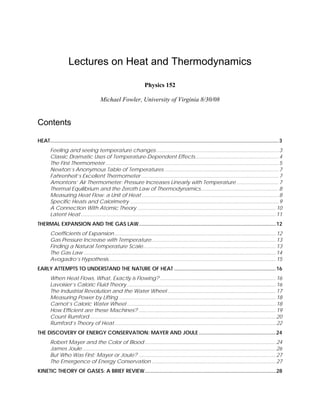
24. 24
discoveries in improving living standards, but also train working class men to become mechanics.
This became the Royal Institution. Unfortunately, Rumford was difficult to work with, and he did
not see eye to eye with the first director, a young Cornishman called Humphry Davy. Sad to report,
Rumford’s idealistic notions for schooling the poor and improving living standards did not become
a priority for the Institution, except for a series of lectures for the public which evolved into
entertainments for the wealthy. Nevertheless, the Institution did maintain a first class laboratory in
which Davy discovered new elements, including sodium and potassium, and has in fact been an
excellent center of scientific research for the last two hundred years. (Check it out here!)
One more remarkable turn of events in Rumford’s life is worth mentioning. Lavoisier, founder of
the caloric theory, was beheaded by French revolutionaries in 1794, leaving a very attractive widow.
Rumford married her in 1805. Perhaps not too surprisingly, the marriage didn’t go well.
In writing the above section, I used mainly the biography Benjamin Thompson, Count Rumford, by
Sanford C. Brown, MIT 1979. I have only been able to mention a small number from the
extraordinary range of Rumford’s inventions (and adventures!) described in this book.
A more recent brief but readable biography: Count Rumford: The Extraordinary Life of a
Scientific Genius, by G. I. Brown, Sutton (UK) 1999.
The Discovery of Energy Conservation: Mayer and Joule
Robert Mayer and the Color of Blood
Julius Robert Mayer was born in the mill town of Heilbronn, Germany, on the river Neckar, in
1814. The town’s whole economy was based on water power. The ten year old Mayer had a
great idea: why not use part of a water wheel’s output to drive an Archimedean screw which
would pump the water back up again? That way you wouldn’t have to rely on the river at all!
Archimedes’ Screw (Wikimedia Commons)

25. 25
He decided to build a model. His first try didn’t work—some water was pumped back up, but
not enough. But surely that could be taken care of by putting in a gear train to make the screw
run faster? Disappointingly, he found the water wheel had a tougher time turning the screw
faster, and he needed to supply a lot more water over the wheel, so he was back to square one.
Increasingly ingenious but unsuccessful fixes finally convinced him that in fact there was no
solution: there was no way to arrange a machine to do work for nothing. This lesson stayed with
Mayer for life.
Mayer studied to become a medical doctor (his studies included one physics course) and in 1840,
at age 25, he signed on as a ship’s doctor on a ship bound for the tropics. Shortly after reaching
the Dutch East Indies, some of the sailors became ill and Mayer’s treatment included blood
letting. He was amazed to find that the venous blood was a bright red, almost the same as arterial
blood. Back in Germany, the venous blood was much darker, and there was a reason: the
chemist Lavoisier had explained that the body’s use of food, at least in part, amounted to burning
it in a controlled way to supply warmth. The darker venous blood in effect contained the ashes,
to be delivered to the lungs and expelled as carbon dioxide. Mayer concluded that less burning
of food was needed to keep warm in the tropics, hence the less dark blood.
Now, Lavoisier had claimed that the amount of heat generated by burning, or oxygenation, of a
certain amount of carbon did not depend on the sequence of chemical reactions involved, so the
heat generated by blood chemistry oxygenation would be the same as that from uncontrolled old-
fashioned burning in air. This quantitative formulation led Mayer to think about how he would
measure the heat generated in the body, to equate it to the food burned. But this soon led to a
problem. Anyone can generate extra heat, just by rubbing the hands together, or, for example, by
turning a rusty, unoiled wheel: the axle will get hot. Does this ‘outside’ heat also count as
generated by the food? Presumably yes, the food powers the body, and the body generates the
heat, even if indirectly. Mayer was convinced from his childhood experience with the water
wheel that nothing came from nothing: that outside heat could not just appear from nowhere, it
had to have a cause.
But he saw that if the indirectly generated heat must also be included, there is a problem. His
analysis ran something like this (I’ve changed the illustration slightly, but the idea’s the same):
suppose two people are each steadily turning large wheels at the same rate, and the wheels are
equally hard to turn. One of them is our rusty unoiled wheel from the last paragraph, and all that
person’s efforts are going into generating heat. But the other wheel has a smooth, oiled axle and
generates a negligible amount of heat. It is equally hard to turn, though, because it is raising a
large bucket of water from a deep well. How do we balance the ‘food = heat’ budget in this
second case?

26. 26
Mayer was forced to the conclusion that for the ‘food = heat’ equation to make sense, there had
to be another equivalence: a certain amount of mechanical work, measured for example by
raising a known weight through a given distance, had to count the same as a certain amount of
heat, measured by raising the temperature of a fixed amount of water, say, a certain number of
degrees. In modern terms, a joule has to be equivalent to a fixed number of calories. Mayer was
the first to spell out this ‘mechanical equivalent of heat’ and in 1842 he calculated the number
using results of experiments done earlier in France on the specific heats of gases. French
experimenters had measured the specific heat of the same gas at constant pressure (Cv) and at
constant pressure (Cp). They always found Cp to be greater than Cv. Mayer interpreted this with
the following thought experiment: consider two identical vertical cylinders, closed at the top by
moveable pistons, the pistons resting on the gas pressure, each enclosing the same amount of the
same gas at the same temperature. Now supply heat to the two gases, for one gas keep the piston
fixed, for the other allow it to rise. Measure how much heat is needed to raise the gas
temperature by ten degrees, say. It is found that extra heat is needed for the gas at constant
pressure, the one where the piston was allowed to rise. Mayer asserted this was because in that
case, some of the heat had been expended as work to raise the piston: this followed very
naturally from his previous thinking, and the French measurements led to a numerical value for
the equivalence. Mayer understood the sequence: a chemical reaction produces heat and work,
that work can then produce a definite amount of heat. This amounted to a statement of the
conservation of energy. Sad to report, Mayer was not part of the German scientific
establishment, and this ground-breaking work was ignored for some years.
James Joule
Meanwhile, in Manchester, England, the center of the industrial revolution, the same problem
was being approached from quite a different direction by James Joule, the son of a prosperous
brewer. Joule was lucky in that as a teenager, he was tutored at home, along with his brother, by
John Dalton, the chemist who founded the atomic theory. Manchester was at the cutting edge of
technological progress, and one exciting idea in the 1830’s was that perhaps coal-driven steam
engines could be replaced by battery-driven electric motors. Joule, in his twenties, set himself the
task of improving the electric motor to the point where it would be competitive with the steam
engine. But it was not to be—after years of effort, he concluded that at best it would take five
pounds of zinc consumed in a battery to deliver the work from one pound of coal. But he learned
a lot. He found an electric current in a wire produced heat at a rate I 2
R, now known as Joule
heating. The caloric theory interpretation was that caloric fluid originally in the battery was
released along with the electric current and settled in the wire. However, Joule discovered the
same heating took place with a current generated by moving the wire past a permanent magnet.
It was difficult to see how the caloric fluid got into the wire in that situation. Joule decided the
caloric theory was suspect. He generated a current by applying a measured force to a dynamo,
and established that the heat appearing in the wire was always directly proportional to the work
done by the force driving the dynamo.

27. 27
Finally, it dawned on him that the electrical intermediary was unnecessary: the heat could be
produced directly by the force, if instead of turning a dynamo, it turned paddle wheels churning
water in an insulated can. The picture below shows his apparatus:
The paddle wheels turn through holes cut in
stationary brass sheets, churning up the water. This is
all inside an insulated can, of course. In this way,
Joule measured the mechanical equivalent of heat,
the same number Mayer had deduced from the
French gas experiments.
Joule’s initial reception by the scientific
establishment was not too different from Mayer’s.
He, too, was a provincial, with a strange accent. But
he had a lucky break in 1847, when he reported his
work to a meeting of the British Association, and
William Thomson was in the audience. Thomson had
just spent a year in Paris. He was fully familiar with
Carnot’s work, and believed the caloric theory to be
correct. But he knew that if Joule really had
produced heat by stirring water, the caloric theory must be wrong—he said there were
‘insuperable difficulties’ in reconciling the two.
But Who Was First: Mayer or Joule?
Mayer and Joule, using entirely different approaches, arrived almost simultaneously at the
conclusion that heat and mechanical work were numerically equivalent: a given amount of work
could be transformed into a quantitatively predictable amount of heat. Which of the two men
deserves more credit (not to mention other contenders!) has been argued for well over a century.
Briefly, it is generally conceded that Mayer was the first to spell out the concept of the
mechanical equivalent of heat (although closely followed, independently, by Joule) and Joule
was the first to put it on a firm experimental basis.
The Emergence of Energy Conservation
In fact, by the 1840’s, although many still believed in the caloric theory, it had run into other
difficulties. Before the 1820’s, almost everyone believed, following Newton, that light was a
stream of particles. Around 1800, Herschel discovered that on passing sunlight through a prism,
and detecting the heat corresponding to the different colors, in fact there was heat transmitted
beyond the red. This suggested that radiant heat was caloric particles streaming through space,
and no doubt very similar in character to light. But in the 1820’s it was unambiguously

28. 28
established that light was really a wave. Did this mean heat was a wave too? Perhaps the caloric
fluid was oscillations in the ether. Things were now very confused. In 1841, Joule wrote
diplomatically: ‘let the space between these compound atoms be supposed to be filled with
calorific ether in a state of vibration, or, otherwise, to be occupied with the oscillations of the
atoms themselves’ (Joule 1963, p.52).
It transpired, though, that the difficulties in reconciling Carnot’s theory and Joule’s experiments
were not as insuperable as Thomson had claimed. In 1850, a German professor, Rudolph
Clausius, pointed out that Carnot’s theory was still almost right: the only adjustment needed was
that there was a little less heat emerging from the bottom of the ‘caloric water wheel’ than went
in at the top—some of the heat became mechanical energy, the work the steam engine was
performing. For real steam engines, the efficiency—the fraction of ingoing heat delivered as
useful work—was so low that it was easy to understand why Carnot’s picture had been accepted
for so long. For the first time, with Clausius’ paper, a coherent theory of heat emerged, and the
days of the caloric theory drew to a close.
Books I used in writing these notes…
Caneva, K. L.: 1993, Robert Mayer and the Conservation of Energy, Princeton University Press,
Princeton, New Jersey.
Cardwell, D. S. L.: 1989, James Joule: A Biography, Manchester University Press, Manchester
and New York.
Cardwell, D. S. L.: 1971, From Watt to Clausius, Cornell University Press, Ithaca, New York.
Joule, J. P.: 1963, Scientific Papers, Vol. I, Dawsons of Pall Mall, London.
Magie, W. F.: 1935, A Source Book in Physics, McGraw-Hill, New York.
Roller, D.: 1957, ‘The Early Development of the Concepts of Temperature and Heat: The Rise
and Decline of the Caloric Theory’, in J. B. Conant and L. K. Nash (eds.), Harvard Case
Histories in Experimental Science, Harvard University Press, Cambridge, Massachusetts, 1957,
117-215.
Kinetic Theory of Gases: A Brief Review
Bernoulli's Picture
Daniel Bernoulli, in 1738, was the first to understand air
pressure from a molecular point of view. He drew a
picture of a vertical cylinder, closed at the bottom, with a
piston at the top, the piston having a weight on it, both
piston and weight being supported by the air pressure
inside the cylinder. He described what went on inside the
cylinder as follows: “let the cavity contain very minute
corpuscles, which are driven hither and thither with a v
rapid motion; so that these corpuscles, when they strike
ery

29. 29
against the piston and sustain it by their repeated impacts, form an elastic fluid which will
expand of itself if the weight is removed or diminished…” (An applet is available here.) Sad to
report, his insight, although essentially correct, was not widely accepted.
Most scientists believed that the molecules in a gas stayed more or less in place, repelling each
other from a distance, held somehow in the ether. Newton had shown that PV = constant
followed if the repulsion were inverse-square. In fact, in the 1820’s an Englishman, John
Herapath, derived the relationship between pressure and molecular speed given below, and tried
to get it published by the Royal Society. It was rejected by the president, Humphry Davy, who
pointed out that equating temperature with motion, as Herapath did, implied that there would be
an absolute zero of temperature, an idea Davy was reluctant to accept. And it should be added
that no-one had the slightest idea how big atoms and molecules were, although Avogadro had
conjectured that equal volumes of different gases at the same temperature and pressure contained
equal numbers of molecules—his famous number—neither he nor anyone else knew what that
number was, only that it was pretty big.
The Link between Molecular Energy and Pressure
It is not difficult to extend Bernoulli’s picture to a quantitative description, relating the gas
pressure to the molecular velocities. As a warm up exercise, let us consider a single perfectly
elastic particle, of mass m, bouncing rapidly back and forth at speed v inside a narrow cylinder of
length L with a piston at one end, so all motion is along the same line. (For the movie, click
here!) What is the force on the piston?
Obviously, the piston doesn’t feel a smooth continuous force, but a series of equally spaced
impacts. However, if the piston is much heavier than the particle, this will have the same effect
as a smooth force over times long compared with the
interval between impacts. So what is the value of the
equivalent smooth force?
v
L
Using Newton’s law in the form force = rate of change of
momentum, we see that the particle’s momentum changes
by 2mv each time it hits the piston. The time between hits is
2L/v, so the frequency of hits is v/2L per second. This m
that if there were no balancing force, by conservation of
momentum the particle would cause the momentum of the
piston to change by 2mv×v/2L units in each second. This is
the rate of change of momentum, and so must be equal to
the balancing force, which is therefore F = mv
eans
2
/L.
We now generalize to the case of many particles bouncing
around inside a rectangular box, of length L in the x-
1-D gas: particle bounces
between ends of cylinder

30. 30
direction (which is along an edge of the box). The total force on the side of area A perpendicular
to the x-direction is just a sum of single particle terms, the relevant velocity being the component
of the velocity in the x-direction. The pressure is just the force per unit area, P = F/A. Of course,
we don’t know what the velocities of the particles are in an actual gas, but it turns out that we
don’t need the details. If we sum N contributions, one from each particle in the box, each
contribution proportional to vx
2
for that particle, the sum just gives us N times the average value
of vx
2
. That is to say,
2 2
/ /x xP F A Nmv LA Nmv V= = = /
where there are N particles in a box of volume V. Next we note that the particles are equally
likely to be moving in any direction, so the average value of vx
2
must be the same as that of vy
2
or
vz
2
, and since v2
= vx
2
+ vy
2
+ vz
2
, it follows that
2
/3 .P Nmv V=
This is a surprisingly simple result! The macroscopic pressure of a gas relates directly to the
average kinetic energy per molecule. Of course, in the above we have not thought about possible
complications caused by interactions between particles, but in fact for gases like air at room
temperature these interactions are very small. Furthermore, it is well established experimentally
that most gases satisfy the Gas Law over a wide temperature range:
PV = nRT
for n moles of gas, that is, n = N/NA, with NA Avogadro’s number and R the gas constant.
Introducing Boltzmann’s constant k = R/NA, it is easy to check from our result for the pressure
and the ideal gas law that the average molecular kinetic energy is proportional to the absolute
temperature,
2 31
2 2 .KE mv k= = T
Boltzmann’s constant k = 1.38.10-23
joules/K.
Maxwell finds the Velocity Distribution
By the 1850’s, various difficulties with the existing theories of heat, such as the caloric theory,
caused some rethinking, and people took another look at the kinetic theory of Bernoulli, but little
real progress was made until Maxwell attacked the problem in 1859. Maxwell worked with
Bernoulli’s picture, that the atoms or molecules in a gas were perfectly elastic particles, obeying
Newton’s laws, bouncing off each other (and the sides of the container) with straight-line
trajectories in between collisions. (Actually, there is some inelasticity in the collisions with the
sides—the bouncing molecule can excite or deexcite vibrations in the wall, this is how the gas

31. 31
and container come to thermal equilibrium.) Maxwell realized that it was completely hopeless to
try to analyze this system using Newton’s laws, even though it could be done in principle, there
were far too many variables to begin writing down equations. On the other hand, a completely
detailed description of how each molecule moved was not really needed anyway. What was
needed was some understanding of how this microscopic picture connected with the macroscopic
properties, which represented averages over huge numbers of molecules.
The relevant microscopic information is not knowledge of the position and velocity of every
molecule at every instant of time, but just the distribution function, that is to say, what
percentage of the molecules are in a certain part of the container, and what percentage have
velocities within a certain range, at each instant of time. For a gas in thermal equilibrium, the
distribution function is independent of time. Ignoring tiny corrections for gravity, the gas will be
distributed uniformly in the container, so the only unknown is the velocity distribution function.
Velocity Space
What does a velocity distribution function look like? Suppose at some instant in time one
particular molecule has velocity ( ), , .x y zv v v v= We can record this information by constructing a
three-dimensional velocity space, with axes , ,x y zv v v , and putting in a point P1 representing the
molecule’s velocity (the red arrow is of coursev ):
vx axis
vy axis
vz axis P1 (vx, vy, vz)
Point P1 represents the location of one molecule in velocity space
Now imagine that at that instant we could measure the velocities of all the molecules in a
container, and put points P2, P3, P4, … PN in the velocity space. Since N is of order 1021
for
100 ccs of gas, this is not very practical! But we can imagine what the result would be: a cloud
of points in velocity space, equally spread in all directions (there’s no reason molecules would
prefer to be moving in the x-direction, say, rather than the y-direction) and thinning out on going
away from the origin towards higher and higher velocities.

32. 32
Now, if we could keep monitoring the situation as time passes individual points would move
around, as molecules bounced off the walls, or each other, so you might think the cloud would
shift around a bit. But there’s a vast number of molecules in any realistic macroscopic situation,
and for any reasonably sized container it’s safe to assume that the number of molecules in any
small region of velocity space remains pretty much constant. Obviously, this cannot be true for a
region of velocity space so tiny that it only contains one or two molecules on average. But it can
be shown statistically that if there are N molecules in a particular small volume of velocity space,
the fluctuation of the number with time is of order N , so a region containing a million
molecules will vary in numbers by about one part in a thousand, a trillion molecule region by one
part in a million. Since 100 ccs of air contains of order 1021
molecules, we can in practice divide
the region of velocity space occupied by the gas into a billion cells, and still have variation in
each cell of order one part in a million!
The bottom line is that for a macroscopic amount of gas, fluctuations in density, both in ordinary
space and in velocity space, are for all practical purposes negligible, and we can take the gas to
be smoothly distributed in both spaces.
Maxwell’s Symmetry Argument
Maxwell found the velocity distribution function for gas molecules in thermal equilibrium by the
following elegant argument based on symmetry.
For a gas of N particles, let the number of particles having velocity in the x-direction between vx
and vx + dvx be ( )1 x xNf v dv . In other words, ( )1 x xf v dv is the fraction of all the particles having
x-direction velocity lying in the interval between vx and vx + dvx. (I’ve written f1 instead of f to
help remember this function refers to only one component of the velocity vector.)
If we add the fractions for all possible values of vx, the result must of course be 1:
( )1 1.x xf v dv
∞
−∞
=∫
But there’s nothing special about the x-direction—for gas molecules in a container, at least away
from the walls, all directions look the same, so the same function f will give the probability
distributions in the other directions too. It follows immediately that the probability for the
velocity to lie between vx and vx + dvx, vy and vy + dvy, and vz and vz + dvz must be:
( ) ( ) ( ) ( ) ( ) ( )1 1 1 1 1 1x x y y z z x y z x yNf v dv f v dv f v dv Nf v f v f v dv dv dv= z

33. 33
Note that this distribution function, when integrated over all possible values of the three
components of velocity, gives the total number of particles to be N, as it should (since integrating
over each f1(v)dv gives unity).
Next comes the clever part—since any direction is as good as any other direction, the distribution
function must depend only on the total speed of the particle, not on the separate velocity
components. Therefore, Maxwell argued, it must be that:
( ) ( ) ( ) ( )2 2 2
1 1 1x y z x y zf v f v f v F v v v= + +
where F is another unknown function. However, it is apparent that the product of the functions
on the left is reflected in the sum of variables on the right. It will only come out that way if the
variables appear in an exponent in the functions on the left. In fact, it is easy to check that this
equation is solved by a function of the form:
( )
2
1 .xBv
xf v Ae−
=
This curve is called a Gaussian: it’s centered at the origin, and falls off very rapidly as vx
increases. Taking A = B = 1 just to see the shape, we find:
At this point, A and B are arbitrary constants—we shall eventually find their values for an actual
sample of gas at a given temperature. Notice that (following Maxwell) we have put a minus sign
in the exponent because there must eventually be fewer and fewer particles on going to higher
speeds, certainly not a diverging number.
Multiplying together the probability distributions for the three directions gives the distribution in
terms of particle speed v, where v2
= vx
2
+vy
2
+ vz
2
. Since all velocity directions are equally

34. 34
likely, it is clear that the natural distribution function is that giving the number of particles
having speed between v and v + dv.
From the graph above, it is clear that the most likely value of vx is zero. If the gas molecules
were restricted to one dimension, just moving back and forth on a line, then the most likely value
of their speed would also be zero. However, for gas molecules free to move in two or three
dimensions, the most likely value of the speed is not zero. It’s easiest to see this in a two-
dimensional example. Suppose we plot the points P representing the velocities of molecules in a
region near the origin, so the density of points doesn’t vary much over the extent of our plot
(we’re staying near the top of the peak in the one-dimensional curve shown above).
Now divide the two-dimensional space into regions corresponding to equal increments in speed:
0 to , to 2 , 2 to 3 ,v v v v vΔ Δ Δ Δ Δ …
In the two-dimensional space, 2 2
constantx yv v v= + = is a circle, so this division of the plane is
into annular regions between circles whose successive radii are vΔ apart:
Constant speed circles in a two-dimensional example
vx
vy
Each of these annular areas corresponds to the same speed increment vΔ . In particular, the
green area, between a circle of radius 8 vΔ and one of radius 9 vΔ , corresponds to the same speed
increment as the small red circle in the middle, which corresponds to speeds between 0 and vΔ .
Therefore, if the molecular speeds are pretty evenly distributed in this near-the-origin area of the
(vx, vy) plane, there will be a lot more molecules with speeds between 8 vΔ and 9 than
between 0 and —so the most likely speed will not be zero. To find out what it actually is, we
vΔ
vΔ

35. 35
have to put this area argument together with the Gaussian fall off in density on going far from the
origin. We’ll discuss this shortly.
The same argument works in three dimensions—it’s just a little more difficult to visualize.
Instead of concentric circles, we have concentric spheres. All points lying on a spherical surface
centered at the origin correspond to the same speed.
Let us now figure out the distribution of particles as a function of speed. The distribution in the
three-dimensional space ( ), ,x y zv v v is from Maxwell’s analysis
( ) ( ) ( )
( )2 2 2
2
1 1 1
3
3
# of particles in small box
x y z
x y z x y z x y z
B v v v
x y z
Bv
x y z
dv dv dv Nf v f v f v dv dv dv
NA e dv dv dv
NA e dv dv dv
− + +
−
=
=
=
To translate this to the number of particles having speed between v and v dv+ we need to figure
out how many of those little x y zdv dv dv boxes there are corresponding to speeds between v and
. In other words, what is the volume of velocity space between the two neighboring
spheres, both centered at the origin, the inner one with radius v, the outer one infinitesimally
bigger, with radius v ? Since dv is so tiny, this volume is just the area of the sphere
multiplied by dv: that is, .
v dv+
dv+
2
4 v dvπ
Finally, then, the probability distribution as a function of speed is:
2
2 3
( ) 4 .Bv
f v dv v A e dvπ −
=
Of course, our job isn’t over—we still have these two unknown constants A and B. However,
just as for the function ( ) ( )1 ,xf v f v dv is the fraction of the molecules corresponding to speeds
between v and , and all these fractions taken together must add up to 1.v dv+
That is,
( )
0
1.f v dv
∞
=∫
We need the standard result ( )
2
2
0
1/ 4 /Bx
x e dx B Bπ
∞
−
=∫ (a derivation can be found in my 152
Notes on Exponential Integrals), and find:
3 1
4 1
4
A
B B
π
π .=

36. 36
This means that there is really only one arbitrary variable left: if we can find B, this equation
gives us A: that is, 3 34
4 A Bπ
π
= / 2
, and 3
4 Aπ is what appears in ( )f v .
Looking at ( )f v , we notice that B is a measure of how far the distribution spreads from the
origin: if B is small, the distribution drops off more slowly—the average particle is more
energetic. Recall now that the average kinetic energy of the particles is related to the
temperature by 2 31
2 2mv kT= . This means that B is related to the inverse temperature.
In fact, since ( )f v dv is the fraction of particles in the interval dv at v, and those particles have
kinetic energy ½mv2
, we can use the probability distribution to find the average kinetic energy
per particle:
2 21 1
2 20
( ) .mv mv f v dv
∞
= ∫
To do this integral we need another standard result: ( )
2
4 2
0
3/8 /Bx
x e dx B Bπ
∞
−
=∫ . We find:
21
2
3
.
4
m
mv
B
=
.Substituting the value for the average kinetic energy in terms of the temperature of the gas,
2 31
2 2mv kT=
gives B = m/2kT, so
3/ 2
3 3/24
4 4
2
m
A B
kT
π π
ππ
⎛ ⎞
= = ⎜ ⎟
⎝ ⎠
.
This means the distribution function
2
3/ 2 3/2
2 /2 2 /
( ) 4 4
2 2
mv kT E kTm m
f v v e v e
kT kT
π π
π π
− −⎛ ⎞ ⎛ ⎞
= =⎜ ⎟ ⎜ ⎟
⎝ ⎠ ⎝ ⎠
where E is the kinetic energy of the molecule.
Note that this function increases parabolically from zero for low speeds, then curves round to
reach a maximum and finally decreases exponentially. As the temperature increases, the position
of the maximum shifts to the right. The total area under the curve is always one, by definition.
For air molecules (say, nitrogen) at room temperature the curve is the blue one below. The red
one is for an absolute temperature down by a factor of two:

37. 37
Michael Fowler, UVa
The distribution function for molecular speeds
as a function of absolute temperature is:
Enter mass and temperature below:
molecular mass:
f v v
m
kT
e mv kT
( ) /
=
F
HG I
KJ −
4
2
2 2
3
2
2
π
π
28
300
517
amu
temperature: K
Boltzmann's const: 1.38E-23 joules/K
1 amu: 1.66E-27 kg
rms speed: m per sec
0
0.0005
0.001
0.0015
0.002
0.0025
0.003
0 200 400 600 800 1000 1200
molecular speed in meters per sec
What about Potential Energy?
Maxwell’s analysis solves the problem of finding the statistical velocity distribution of molecules
of an ideal gas in a box at a definite temperature T: the relative probability of a molecule having
velocity is proportional to . The position distribution is taken to be uniform:
the molecules are assumed to be equally likely to be anywhere in the box.
v
2
/2 /mv kT E kT
e e− −
=
But how is this distribution affected if in fact there is some kind of potential pulling the
molecules to one end of the box? In fact, we’ve already solved this problem, in the discussion
earlier on the isothermal atmosphere. Consider a really big box, kilometers high, so air will be
significantly denser towards the bottom. Assume the temperature is uniform throughout. We
found under these conditions that with Boyles Law expressed in the form
CPρ =
the atmospheric density varied with height as
0 0, or equivalently .Cgh Cgh
P P e eρ ρ− −
= =
Now we know that Boyle’s Law is just the fixed temperature version of the Gas Law PV nRT= ,
and the density
mass/volume /Nm Vρ = =

38. 38
with N the total number of molecules and m the molecular mass,
/ .CP Nm Vρ= =
Rearranging,
/ /APV Nm C nN m C,= =
for n moles of gas, each mole containing Avogadro’s number NA molecules.
Putting this together with the Gas Law,
/ ,APV nN m C nRT= =
So
/ /AC N m RT m kT= =
where Boltzmann’s constant as discussed previously./ Ak R N=
The dependence of gas density on height can therefore be written
/
0 0 .Cgh mgh kT
e eρ ρ ρ− −
= =
The important point here is that mgh is the potential energy of the molecule, and the distribution
we have found is exactly parallel to Maxwell’s velocity distribution, the potential energy now
playing the role that kinetic energy played in that case.
We’re now ready to put together Maxwell’s velocity distribution with this height distribution, to
find out how the molecules are distributed in the atmosphere, both in velocity space and in
ordinary space. In other words, in a six-dimensional space!
Our result is:
( ) ( )
( )( )22 1/2 //2 / /
, , , , , , .
mv mgh kTmv kT mgh kT E kT
x y zf x y z v v v f h v e e e e
− +− − −
= ∝ = =
That is, the probability of a molecule having total energy E is proportional to ./E kT
e−
This is the Boltzmann, or Maxwell-Boltzmann, distribution. It turns out to be correct for any
type of potential energy, including that arising from forces between the molecules themselves.

39. 39
Degrees of Freedom and Equipartition of Energy
By a “degree of freedom” we mean a way in which a molecule is free to move, and thus have
energy—in this case, just the x, y, and z directions. Boltzmann reformulated Maxwell’s analysis
in terms of degrees of freedom, stating that there was an average energy ½kT in each degree of
freedom, to give total average kinetic energy 3.½kT, so the specific heat per molecule is
presumable 1.5k, and given that k = R/NA, the specific heat per mole comes out at 1.5R. In fact,
this is experimentally confirmed for monatomic gases. However, it is found that diatomic gases
can have specific heats of 2.5R and even 3.5R. This is not difficult to understand—these
molecules have more degrees of freedom. A dumbbell molecule can rotate about two directions
perpendicular to its axis. A diatomic molecule could also vibrate. Such a simple harmonic
oscillator motion has both kinetic and potential energy, and it turns out to have total energy kT
in thermal equilibrium. Thus, reasonable explanations for the specific heats of various gases can
be concocted by assuming a contribution ½k from each degree of freedom. But there are
problems. Why shouldn’t the dumbbell rotate about its axis? Why do monatomic atoms not
rotate at all? Even more ominously, the specific heat of hydrogen, 2.5R at room temperature,
drops to 1.5R at lower temperatures. These problems were not resolved until the advent of
quantum mechanics.
Brownian Motion
One of the most convincing demonstrations that gases really are made up of fast moving
molecules is Brownian motion, the observed constant jiggling around of tiny particles, such as
fragments of ash in smoke. This motion was first noticed by a Scottish botanist, who initially
assumed he was looking at living creatures, but then found the same motion in what he knew to
be particles of inorganic material. Einstein showed how to use Brownian motion to estimate the
size of atoms. For the movie, click here!
Ideal Gas Thermodynamics: Specific Heats, Isotherms,
Adiabats
Introduction: the Ideal Gas Model, Heat, Work and Thermodynamics
The Kinetic Theory picture of a gas (outlined in the previous lecture) is often called the Ideal
Gas Model. It ignores interactions between molecules, and the finite size of molecules. In fact,
though, these only become important when the gas is very close to the temperature at which it
become liquid, or under extremely high pressure. In this lecture, we will be analyzing the
behavior of gases in the pressure and temperature range corresponding to heat engines, and in
this range the Ideal Gas Model is an excellent approximation. Essentially, our program here is to
learn how gases absorb heat and turn it into work, and vice versa. This heat-work interplay is
called thermodynamics.

40. 40
Julius Robert Mayer was the first to appreciate that there is an equivalence between heat and
mechanical work. The tortuous path that led him to this conclusion is described in an earlier
lecture, but once he was there, he realized that in fact the numerical equivalence—how many
Joules in one calorie in present day terminology—could be figured out easily from the results of
some measurements of gas specific heat by French scientists. The key was that they had
measured specific heats both at constant volume and at constant pressure. Mayer realized that in
the latter case, heating the gas necessarily increased its volume, and the gas therefore did work in
pushing to expand its container. Having convinced himself that mechanical work and heat were
equivalent, evidently the extra heat needed to raise the temperature of the gas at constant
pressure was exactly the work the gas did on its container. (Historical note: although he did the
work in 1842, he didn’t publish until 1845, and at first miscalculated—but then gave a figure
within 1% of the correct value of 4.2 joules per calorie.)
The simplest way to see what’s going on is to imagine the gas in a cylinder, held in by a piston,
carrying a fixed weight, able to move up and down the cylinder smoothly with negligible
friction. The pressure on the gas is just the total weight pressing down divided by the area of the
piston, and this total weight, of course, will not change as the piston moves slowly up or down:
the gas is at constant pressure.
Moveable
piston
Gas
Gas at constant pressure
The Gas Specific Heats CV and CP
Consider now the two specific heats of this same sample of gas, let’s say one mole:
Specific heat at constant volume, (piston glued in place),VC
Specific heat at constant pressure, PC (piston free to rise, no friction).