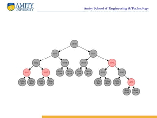
Hashing in data base managementsystem_Updated.pptx
1.
Amity School ofEngineering & Technology
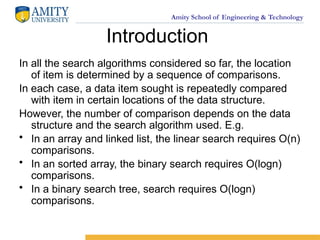
Introduction
In all the search algorithms considered so far, the location
of item is determined by a sequence of comparisons.
In each case, a data item sought is repeatedly compared
with item in certain locations of the data structure.
However, the number of comparison depends on the data
structure and the search algorithm used. E.g.
• In an array and linked list, the linear search requires O(n)
comparisons.
• In an sorted array, the binary search requires O(logn)
comparisons.
• In a binary search tree, search requires O(logn)
comparisons.
2.
Amity School ofEngineering & Technology
However, there are some applications that
requires search to be performed in
constant time, i.e. O(1).
Ideally it may not be possible, but still we
can achieve a performance very close to
it. And this is possible using a data
structure known as hash table.
3.
Amity School ofEngineering & Technology
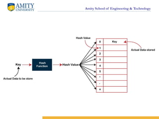
What is hash function?
• A hash function h is simply a mathematical
formula that manipulates the key in some form
to compute the index for this key in the hash
table.
For example, a hash function can divide the key
by some number, usually size of the hash table,
and return remainder as the index of the key.
• In general, we say that a hash function h maps
the universe U of keys into the slots of a hash
table T[0..m-1]. This process of mapping keys
to appropriate slots in a hash table is known as
hashing.
4.
Amity School ofEngineering & Technology
Different hash functions
• There is variety of hash functions.
The main considerations while choosing
particular hash function h are:
1. It should be possible to compute it
efficiently
2. It should distribute the keys uniformly
across the hash table i.e. it should keep
the number of collisions as minimum as
possible.
Amity School ofEngineering & Technology
Hash Functions
1. Division method:
In division method, key K to be mapped into
one of the m slots in the hash table is
divided by m and the remainder of this
division is taken as index into the hash
table.
That is hash function is
h(k)=k mod m
7.
Amity School ofEngineering & Technology
Division method
Consider a hash table with 9 slots i.e. m=9
then the hash function
h(k)= k mod m
will map the key 132 to slot 6 since
h(132)= 132 mod 9 = 6
Since it requires only a single division
operation, hashing is quite fast.
8.
Amity School ofEngineering & Technology
example
• Let company has 90 employees and 00,01,02,..89 be
the two digits 90 memory address ( or index or hash
address) to store the records. We have employee
code as the key.
• Choose m in such a way that it is greater than 90.
suppose m=93, then for the following employee code
(or key k)
h(k)=h(2103)=2103(mod 93) =57
h(k)=h(6147)=6147(mod 93) =9
h(k)=h(3750)=3750(mod 93) =30
Then typical hash table will look like as next page
So if you enter the employee code to the hash function
we can directly retrieve table[h[k]] details directly.
9.
Amity School ofEngineering & Technology
Midsquare method
• The midsquare method operates in two step, the
square of the key value k is taken. In the second
step, the hash value is obtained by deleting
digits from ends of the squared value i.e.k2
. It is
important to note that same position of k2
must
be used for all keys. This the hash function is
h(k)=s
Where s is obtained by deleting digits from both
sides of k2
.
10.
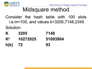
Amity School ofEngineering & Technology
Midsquare method
Consider the hash table with 100 slots
i.e.m=100, and values k=3205,7148,2345
Solution:
K 3205 7148
K2
10272025 51093904
h(k) 72 93
11.
Amity School ofEngineering & Technology
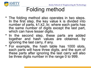
Folding method
• The folding method also operates in two steps.
In the first step, the key value k is divided into
number of parts, k1,k2..kr, where each parts has
the same number of digits except the last part,
which can have lesser digits.
• In the second step, these parts are added
together and hash values are obtained. by
ignoring the last carry, if any.
• For example, the hash table has 1000 slots,
each parts will have three digits, and the sum of
these parts after ignoring the last carry will also
be three digits number in the range 0 to 999.
12.
Amity School ofEngineering & Technology
H (7148) = 71 + 84 = 55
H (2345) = 23 + 45 = 68
13.
Amity School ofEngineering & Technology
Collision
When the two different values have the
same value, then the problem occurs
between the two values, known as a
collision.
14.
Amity School ofEngineering & Technology
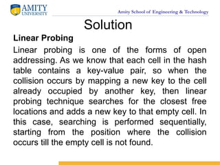
Solution
Linear Probing
Linear probing is one of the forms of open
addressing. As we know that each cell in the hash
table contains a key-value pair, so when the
collision occurs by mapping a new key to the cell
already occupied by another key, then linear
probing technique searches for the closest free
locations and adds a new key to that empty cell. In
this case, searching is performed sequentially,
starting from the position where the collision
occurs till the empty cell is not found.
15.
Amity School ofEngineering & Technology
Chaining method:-
1. Using Array
2. Using Linked List
16.
Amity School ofEngineering & Technology
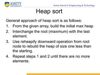
Heap sort
General approach of heap sort is as follows:
1. From the given array, build the initial max heap
2. Interchange the root (maximum) with the last
element.
3. Use reheapify downward operation from root
node to rebuild the heap of size one less than
the starting.
4. Repeat steps 1 and 2 until there are no more
elements.
Amity School ofEngineering & Technology
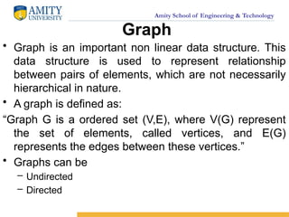
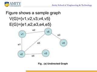
Graph
• Graph is an important non linear data structure. This
data structure is used to represent relationship
between pairs of elements, which are not necessarily
hierarchical in nature.
• A graph is defined as:
“Graph G is a ordered set (V,E), where V(G) represent
the set of elements, called vertices, and E(G)
represents the edges between these vertices.”
• Graphs can be
– Undirected
– Directed
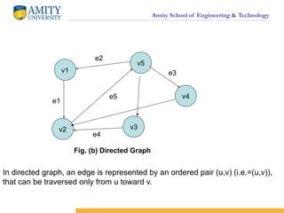
Amity School ofEngineering & Technology
v1
v5
v4
v2 v3
e2
e1
e5
e4
e3
Fig. (b) Directed Graph
In directed graph, an edge is represented by an ordered pair (u,v) (i.e.=(u,v)),
that can be traversed only from u toward v.
21.
Amity School ofEngineering & Technology
• Adjacent Vertices:
As an edge e is represented by pairs of vertices
denoted by [u,v]. The vertices u and v are called
endpoints of e. these vertices are also called
adjacent vertices or neighbors.
• Degree of a vertex:
The degree of vertex u, written as deg(u), is the
number of edges containing u. If deg(u)=0, this
means that vertex u does not belong to any
edge, then vertex u is called an isolated vertex.
22.
Amity School ofEngineering & Technology
• Path:
A path P of length n from a vertex u to vertex v is defined
as sequence of (n+1) vertices i.e.
P=(v1,v2,v3,……vn+1)
Such that u=v1, v=vn+1
• The path is said to be closed if the endpoints of the
path are same i.e. v1=vn+1.
• The path is said to be simple if all the vertices in the
sequence are distinct, with the exception that
v1=vn+1.In that case it is known as closed simple path.
23.
Amity School ofEngineering & Technology
• Cycle:
A cycle is closed simple path with length two or
more. Sometimes, a cycle of length k (i.e. k
distinct vertices in the path) is known as k-cycle.
• Connected Graph:
A graph is said to be connected if there is path
between any two of its vertices, i.e. there is no
isolated vertex.
A connected graph without any cycles is called
a tree. Thus we can say that tree is a special
graph.
24.
Amity School ofEngineering & Technology
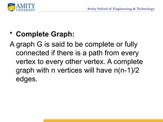
• Complete Graph:
A graph G is said to be complete or fully
connected if there is a path from every
vertex to every other vertex. A complete
graph with n vertices will have n(n-1)/2
edges.
25.
Amity School ofEngineering & Technology
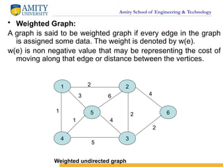
• Weighted Graph:
A graph is said to be weighted graph if every edge in the graph
is assigned some data. The weight is denoted by w(e).
w(e) is non negative value that may be representing the cost of
moving along that edge or distance between the vertices.
1 2
4 3
5 6
2
5
1
3 6
1 4
4
2
2
Weighted undirected graph
26.
Amity School ofEngineering & Technology
Representation of Graph
• Using an adjacency matrix
• Using an adjacency list
27.
Amity School ofEngineering & Technology
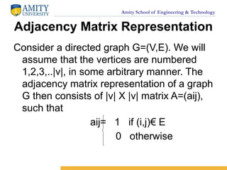
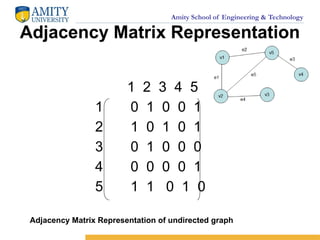
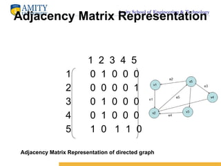
Adjacency Matrix Representation
Consider a directed graph G=(V,E). We will
assume that the vertices are numbered
1,2,3,..|v|, in some arbitrary manner. The
adjacency matrix representation of a graph
G then consists of |v| X |v| matrix A=(aij),
such that
aij= 1 if (i,j)€ E
0 otherwise
28.
Amity School ofEngineering & Technology
Adjacency Matrix Representation
For undirected graph G=(V,E), the
adjacency matrix representation is also
consists of |v|X|v| matrix A=(aij) but its
elements are as follows:
aij= 1 if either [I,j] € E or [j,i] €
E
0 otherwise
Amity School ofEngineering & Technology
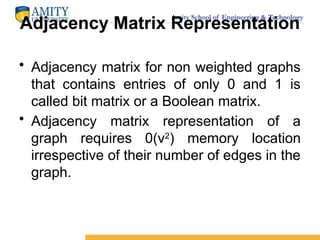
Adjacency Matrix Representation
• Adjacency matrix for non weighted graphs
that contains entries of only 0 and 1 is
called bit matrix or a Boolean matrix.
• Adjacency matrix representation of a
graph requires 0(v2
) memory location
irrespective of their number of edges in the
graph.
32.
Amity School ofEngineering & Technology
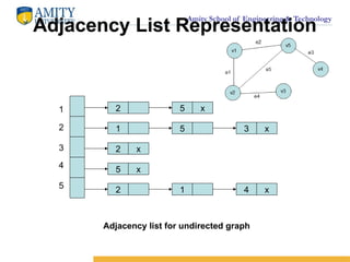
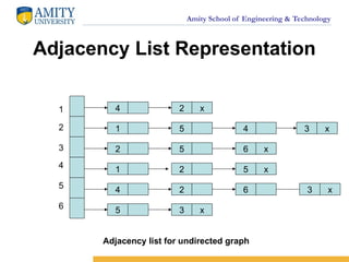
Adjacency List Representation
• The Adjacency List Representation of a
graph G=(V,E) consists of an array Adj of |
V| lists, one for each vertex in V.
• For each u € V , the adjacency list Adj[u]
contains all the vertices v such that there
is an edge (u,v) € E i.e. Adj[u] consists of
all the vertices adjacent to u in G.
• The vertices in each adjacency list are
stored in an arbitrary order.
33.
Amity School ofEngineering & Technology
Adjacency List Representation
2
1
2 x
5 x
2
5 x
5 3 x
1 4 x
1
2
3
4
5
Adjacency list for undirected graph
34.
Amity School ofEngineering & Technology
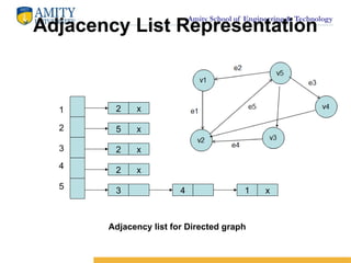
Adjacency List Representation
2 x
5 x
2 x
2 x
3 4 1 x
1
2
3
4
5
Adjacency list for Directed graph
35.
Amity School ofEngineering & Technology
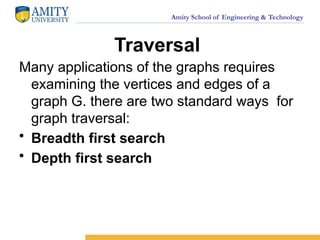
Traversal
Many applications of the graphs requires
examining the vertices and edges of a
graph G. there are two standard ways for
graph traversal:
• Breadth first search
• Depth first search
36.
Amity School ofEngineering & Technology
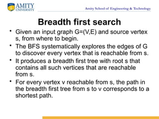
Breadth first search
• Given an input graph G=(V,E) and source vertex
s, from where to begin.
• The BFS systematically explores the edges of G
to discover every vertex that is reachable from s.
• It produces a breadth first tree with root s that
contains all such vertices that are reachable
from s.
• For every vertex v reachable from s, the path in
the breadth first tree from s to v corresponds to a
shortest path.
37.
Amity School ofEngineering & Technology
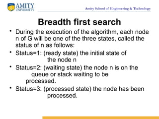
Breadth first search
• During the execution of the algorithm, each node
n of G will be one of the three states, called the
status of n as follows:
• Status=1: (ready state) the initial state of
the node n
• Status=2: (waiting state) the node n is on the
queue or stack waiting to be
processed.
• Status=3: (processed state) the node has been
processed.
38.
Amity School ofEngineering & Technology
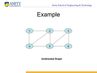
Example
1 2
4 5 6
3
Undirected Graph
39.
Amity School ofEngineering & Technology
Adjacency List Representation
4
1
2
1
4
2 x
5 4
2 6
1
2
3
4
5
Adjacency list for undirected graph
6
3 x
3 x
5 6 x
2 5 x
5 3 x
40.
Amity School ofEngineering & Technology
BFS Algorithm
Step 1:Initialize all nodes to ready state (status =1)
Step 2: Put the starting node in queue and change its
status to the waiting state (status=2)
Step 3: Repeat step 4 and 5 until queue is empty
Step 4: Remove the front node n of queue. Process n
and change the status of n to the processed state
(status=3)
Step 5: Add to the rear of the queue all the neighbor of
n that are in ready state (status=1), and change
their status to the waiting state (status=2)
[end of the step 3 loop]
Step 6: exit
41.
Amity School ofEngineering & Technology
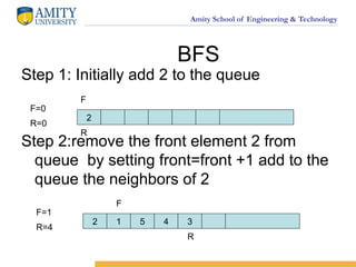
BFS
Step 1: Initially add 2 to the queue
Step 2:remove the front element 2 from
queue by setting front=front +1 add to the
queue the neighbors of 2
2
F=0
R=0
F
R
2 1 5 4 3
F=1
R=4
F
R
42.
Amity School ofEngineering & Technology
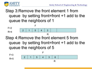
Step 3:Remove the front element 1 from
queue by setting front=front +1 add to the
queue the neighbors of 1
Step 4:Remove the front element 5 from
queue by setting front=front +1 add to the
queue the neighbors of 5
2 1 5 4 3
F=2
R=4
F
R
2 1 5 4 3 6
F=3
R=5
F
R
43.
Amity School ofEngineering & Technology
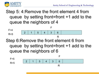
Step 5: 4:Remove the front element 4 from
queue by setting front=front +1 add to the
queue the neighbors of 4
Step 6:Remove the front element 6 from
queue by setting front=front +1 add to the
queue the neighbors of 6
2 1 5 4 3 6
F=4
R=5
F
R
2 1 5 4 3 6
F=5
R=5
F
R
44.
Amity School ofEngineering & Technology
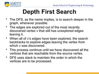
Depth First Search
• The DFS, as the name implies, is to search deeper in the
graph, whenever possible.
• The edges are explored out of the most recently
discovered vertex v that still has unexplored edges
leaving it.
• When all of v’s edges have been explored, the search
backtracks to explore edges leaving the vertex from
which v was discovered.
• This process continue until we have discovered all the
vertices that are reachable from the source vertex.
• DFS uses stack to maintain the order in which the
vertices are to be processed.
45.
Amity School ofEngineering & Technology
Algorithm
Step 1:Initialize all nodes to ready state (status =1)
Step 2: Push the starting node in stack and change its
status to the waiting state (status=2)
Step 3: Repeat step 4 and 5 until stack is empty
Step 4: pop the top node n of stack. Process n and
change the status of n to the processed state (status=3)
Step 5: Push on to stack all the neighbor of n that are
in ready state (status=1), and change their status to
the waiting state (status=2)
[end of the step 3 loop]
Step 6: exit
Amity School ofEngineering & Technology
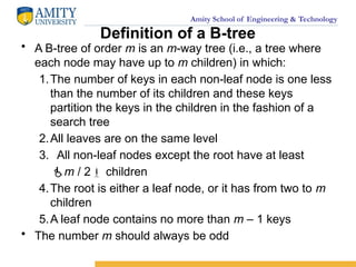
Definition of a B-tree
• A B-tree of order m is an m-way tree (i.e., a tree where
each node may have up to m children) in which:
1.The number of keys in each non-leaf node is one less
than the number of its children and these keys
partition the keys in the children in the fashion of a
search tree
2.All leaves are on the same level
3. All non-leaf nodes except the root have at least
m / 2 children
4.The root is either a leaf node, or it has from two to m
children
5.A leaf node contains no more than m – 1 keys
• The number m should always be odd
48.
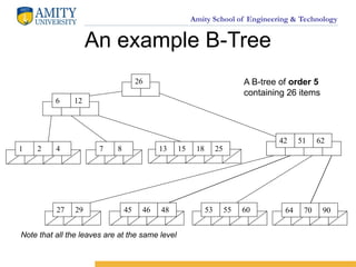
Amity School ofEngineering & Technology
An example B-Tree
51 62
42
6 12
26
55 60 70
64 90
45
1 2 4 7 8 13 15 18 25
27 29 46 48 53
A B-tree of order 5
containing 26 items
Note that all the leaves are at the same level
49.
Amity School ofEngineering & Technology
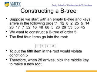
Constructing a B-tree
• Suppose we start with an empty B-tree and keys
arrive in the following order:1 12 8 2 25 5 14
28 17 7 52 16 48 68 3 26 29 53 55 45
• We want to construct a B-tree of order 5
• The first four items go into the root:
• To put the fifth item in the root would violate
condition 5
• Therefore, when 25 arrives, pick the middle key
to make a new root
1 2 8 12
50.
Amity School ofEngineering & Technology
1 2
8
12 25
6, 14, 28 get added to the leaf nodes:
1 2
8
12 14
6 25 28
51.
Amity School ofEngineering & Technology
Adding 17 to the right leaf node would over-fill it, so we take the
middle key, promote it (to the root) and split the leaf
8 17
12 14 25 28
1 2 6
7, 52, 16, 48 get added to the leaf nodes
8 17
12 14 25 28
1 2 6 16 48 52
7
52.
Amity School ofEngineering & Technology
Adding 68 causes us to split the right most leaf, promoting 48 to the
root, and adding 3 causes us to split the left most leaf, promoting 3
to the root; 26, 29, 53, 55 then go into the leaves
3 8 17 48
52 53 55 68
25 26 28 29
1 2 6 7 12 14 16
Adding 45 causes a split of 25 26 28 29
and promoting 28 to the root then causes the root to split
Amity School ofEngineering & Technology
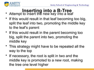
Inserting into a B-Tree
• Attempt to insert the new key into a leaf
• If this would result in that leaf becoming too big,
split the leaf into two, promoting the middle key
to the leaf’s parent
• If this would result in the parent becoming too
big, split the parent into two, promoting the
middle key
• This strategy might have to be repeated all the
way to the top
• If necessary, the root is split in two and the
middle key is promoted to a new root, making
the tree one level higher
55.
Amity School ofEngineering & Technology
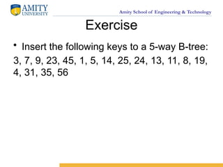
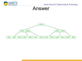
Exercise
• Insert the following keys to a 5-way B-tree:
3, 7, 9, 23, 45, 1, 5, 14, 25, 24, 13, 11, 8, 19,
4, 31, 35, 56
Amity School ofEngineering & Technology
AVL TREES
• We can guarantee O(log2n) performance
for each search tree operation by ensuring
that the search tree height is always
O(log2n).
• Trees with a worst case height of O(log2n)
are called balanced trees.
• One of the popular balanced tree is AVL
tree, which was introduced by Adelson-
Velskii and Landis.
58.
Amity School ofEngineering & Technology
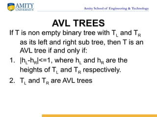
AVL TREES
If T is non empty binary tree with TL and TR
as its left and right sub tree, then T is an
AVL tree if and only if:
1. |hL-hR|<=1, where hL and hR are the
heights of TL and TR respectively.
2. TL and TR are AVL trees
59.
Amity School ofEngineering & Technology
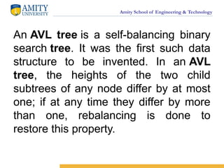
An AVL tree is a self-balancing binary
search tree. It was the first such data
structure to be invented. In an AVL
tree, the heights of the two child
subtrees of any node differ by at most
one; if at any time they differ by more
than one, rebalancing is done to
restore this property.
Amity School ofEngineering & Technology
Representation of AVL trees
The node of the AVL tree is additional field bf (balanced
factor) in addition to the structure to the node in binary
search tree.
struct node
{
struct node *left;
int info;
int bf;
struct node *right;
};
struct node *root;
62.
Amity School ofEngineering & Technology
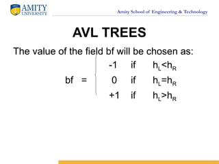
AVL TREES
The value of the field bf will be chosen as:
-1 if hL<hR
bf = 0 if hL=hR
+1 if hL>hR
63.
Amity School ofEngineering & Technology
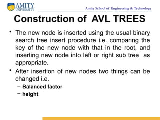
Construction of AVL TREES
• The new node is inserted using the usual binary
search tree insert procedure i.e. comparing the
key of the new node with that in the root, and
inserting new node into left or right sub tree as
appropriate.
• After insertion of new nodes two things can be
changed i.e.
– Balanced factor
– height
64.
Amity School ofEngineering & Technology
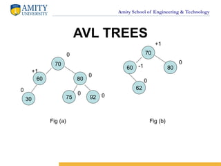
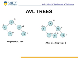
AVL TREES
8
5 10
15
7
0
-1
0
0
-1
8
5 10
15
7
0
0
0
0
-1
9
0
Original AVL Tree
After inserting value 9
65.
Amity School ofEngineering & Technology
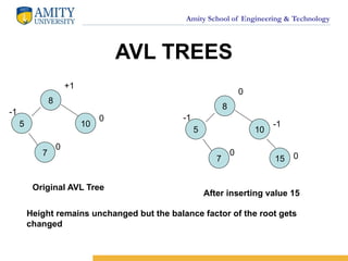
AVL TREES
8
5 10
7
+1
0
0
-1
8
5 10
15
7
0
-1
0
0
-1
Original AVL Tree
After inserting value 15
Height remains unchanged but the balance factor of the root gets
changed
66.
Amity School ofEngineering & Technology
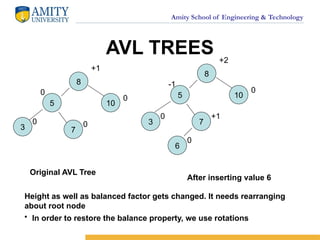
AVL TREES
8
5 10
7
+1
0
0
0
8
5 10
7
+2
0
+1
-1
Original AVL Tree
After inserting value 6
Height as well as balanced factor gets changed. It needs rearranging
about root node
• In order to restore the balance property, we use rotations
3
0 3
0
6
0
67.
Amity School ofEngineering & Technology
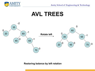
AVL TREES
35
20 60
45
-2
-1
0
0 60
35 65
70
45
0
-1
0
0
0
65
-1
70
0
20
0
Rotate left
Restoring balance by left rotation
68.
Amity School ofEngineering & Technology
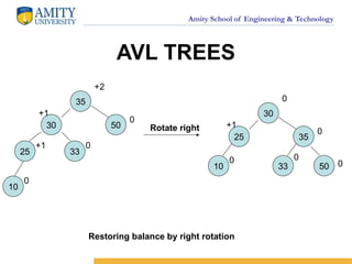
AVL TREES
35
30 50
25
+2
0
+1
+1 30
25 35
50
33
0
0
0
0
+1
33
0
10
0
10
0
Rotate right
Restoring balance by right rotation
69.
Amity School ofEngineering & Technology
Construct AVL Tree
70,80,90,10,5,40,20,50
Amity School ofEngineering & Technology
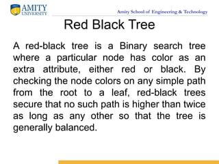
Red Black Tree
A red-black tree is a Binary search tree
where a particular node has color as an
extra attribute, either red or black. By
checking the node colors on any simple path
from the root to a leaf, red-black trees
secure that no such path is higher than twice
as long as any other so that the tree is
generally balanced.
72.
Amity School ofEngineering & Technology
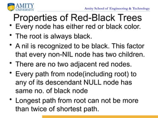
Properties of Red-Black Trees
• Every node has either red or black color.
• The root is always black.
• A nil is recognized to be black. This factor
that every non-NIL node has two children.
• There are no two adjacent red nodes.
• Every path from node(including root) to
any of its descendant NULL node has
same no. of black node
• Longest path from root can not be more
than twice of shortest path.
Amity School ofEngineering & Technology
Red Black Tree Construction
1. If TREE is empty create new node as root node with color Black.
2. If TREE is not empty create new node as leaf node with color Red.
3. If parent of new node is Black then Exit.
4. If parent of new node is Red, Then check the color of parent’s
sibling of new node:-
(a) If color of parent’s sibling is Black or Null then do required
rotation and recolor.
(b) If color of parent’s sibling is Red then recolor(both parent and
its sibling ) and then also check parent’s parent of new node is not root
node then recolor it and re check.
75.
Amity School ofEngineering & Technology
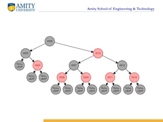
Construct Red Black Tree
5,3,10,4,7,11,6,8,12,15
![Amity School of Engineering & Technology
What is hash function?
• A hash function h is simply a mathematical
formula that manipulates the key in some form
to compute the index for this key in the hash
table.
For example, a hash function can divide the key
by some number, usually size of the hash table,
and return remainder as the index of the key.
• In general, we say that a hash function h maps
the universe U of keys into the slots of a hash
table T[0..m-1]. This process of mapping keys
to appropriate slots in a hash table is known as
hashing.](https://image.slidesharecdn.com/hashingupdated-250510031925-50fd061a/85/Hashing-in-data-base-managementsystem_Updated-pptx-3-320.jpg)
![Amity School of Engineering & Technology
example
• Let company has 90 employees and 00,01,02,..89 be
the two digits 90 memory address ( or index or hash
address) to store the records. We have employee
code as the key.
• Choose m in such a way that it is greater than 90.
suppose m=93, then for the following employee code
(or key k)
h(k)=h(2103)=2103(mod 93) =57
h(k)=h(6147)=6147(mod 93) =9
h(k)=h(3750)=3750(mod 93) =30
Then typical hash table will look like as next page
So if you enter the employee code to the hash function
we can directly retrieve table[h[k]] details directly.](https://image.slidesharecdn.com/hashingupdated-250510031925-50fd061a/85/Hashing-in-data-base-managementsystem_Updated-pptx-8-320.jpg)

![Amity School of Engineering & Technology
• Adjacent Vertices:
As an edge e is represented by pairs of vertices
denoted by [u,v]. The vertices u and v are called
endpoints of e. these vertices are also called
adjacent vertices or neighbors.
• Degree of a vertex:
The degree of vertex u, written as deg(u), is the
number of edges containing u. If deg(u)=0, this
means that vertex u does not belong to any
edge, then vertex u is called an isolated vertex.](https://image.slidesharecdn.com/hashingupdated-250510031925-50fd061a/85/Hashing-in-data-base-managementsystem_Updated-pptx-21-320.jpg)

![Amity School of Engineering & Technology
Adjacency Matrix Representation
For undirected graph G=(V,E), the
adjacency matrix representation is also
consists of |v|X|v| matrix A=(aij) but its
elements are as follows:
aij= 1 if either [I,j] € E or [j,i] €
E
0 otherwise](https://image.slidesharecdn.com/hashingupdated-250510031925-50fd061a/85/Hashing-in-data-base-managementsystem_Updated-pptx-28-320.jpg)
![Amity School of Engineering & Technology
Adjacency List Representation
• The Adjacency List Representation of a
graph G=(V,E) consists of an array Adj of |
V| lists, one for each vertex in V.
• For each u € V , the adjacency list Adj[u]
contains all the vertices v such that there
is an edge (u,v) € E i.e. Adj[u] consists of
all the vertices adjacent to u in G.
• The vertices in each adjacency list are
stored in an arbitrary order.](https://image.slidesharecdn.com/hashingupdated-250510031925-50fd061a/85/Hashing-in-data-base-managementsystem_Updated-pptx-32-320.jpg)
![Amity School of Engineering & Technology
BFS Algorithm
Step 1:Initialize all nodes to ready state (status =1)
Step 2: Put the starting node in queue and change its
status to the waiting state (status=2)
Step 3: Repeat step 4 and 5 until queue is empty
Step 4: Remove the front node n of queue. Process n
and change the status of n to the processed state
(status=3)
Step 5: Add to the rear of the queue all the neighbor of
n that are in ready state (status=1), and change
their status to the waiting state (status=2)
[end of the step 3 loop]
Step 6: exit](https://image.slidesharecdn.com/hashingupdated-250510031925-50fd061a/85/Hashing-in-data-base-managementsystem_Updated-pptx-40-320.jpg)
![Amity School of Engineering & Technology
Algorithm
Step 1:Initialize all nodes to ready state (status =1)
Step 2: Push the starting node in stack and change its
status to the waiting state (status=2)
Step 3: Repeat step 4 and 5 until stack is empty
Step 4: pop the top node n of stack. Process n and
change the status of n to the processed state (status=3)
Step 5: Push on to stack all the neighbor of n that are
in ready state (status=1), and change their status to
the waiting state (status=2)
[end of the step 3 loop]
Step 6: exit](https://image.slidesharecdn.com/hashingupdated-250510031925-50fd061a/85/Hashing-in-data-base-managementsystem_Updated-pptx-45-320.jpg)