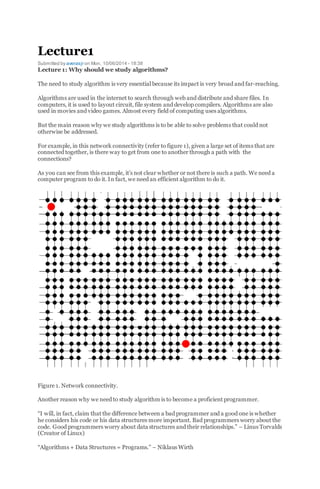
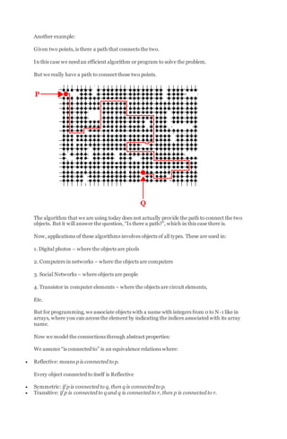
The document discusses algorithms for solving dynamic connectivity problems. It introduces the union-find problem and describes two algorithms - quick find and quick union - for solving it. The key aspects are: 1) The union-find problem involves connecting a set of objects through union commands and checking connectivity through find queries. 2) Developing usable algorithms involves modeling the problem, finding an initial algorithm, and iteratively improving it based on performance and memory usage. 3) The quick find and quick union algorithms use arrays to represent connections between objects and support union and find operations efficiently.

1. Lecture1
Submitted by averasjr on Mon, 10/06/2014 - 18:38
Lecture 1: Why should we study algorithms?
The need to study algorithm is very essential because its impact is very broad and far-reaching.
Algorithms are used in the internet to search through web and distribute and share files. In
computers, it is used to layout circuit, file system and develop compilers. Algorithms are also
used in movies and video games. Almost every field of computing uses algorithms.
But the main reason why we study algorithms is to be able to solve problems that could not
otherwise be addressed.
For example, in this network connectivity (refer to figure 1), given a large set of items that are
connected together, is there way to get from one to another through a path with the
connections?
As you can see from this example, it’s not clear whether or not there is such a path. We need a
computer program to do it. In fact, we need an efficient algorithm to do it.
Figure 1. Network connectivity.
Another reason why we need to study algorithm is to become a proficient programmer.
“I will, in fact, claim that the difference between a bad programmer and a good one is whether
he considers his code or his data structures more important. Bad programmers worry about the
code. Good programmers worry about data structures and their relationships.” – Linus Torvalds
(Creator of Linux)
“Algorithms + Data Structures = Programs.” – Niklaus Wirth

2. Another reason why we need to study algorithms is to unlock secrets of life and of the universe.
Algorithms have become a commonlanguage in understanding nature. Computational models
are replacing mathematical models in scientific inquiry.
In the 20th century, scientist develops mathematical models to try to understand natural
phenomena. However, these mathematical formula or models are very difficult to solve or to
create solutions to be able to test hypothesis against natural phenomenon.
In the 21st century, more and more people are developing computational models where they
attempt to simulate what might be happening in nature in order to try to better understand it.
Algorithms play a very important role in this process.
Another reason why we study algorithms is for fun and profit.
If you are able to know how to effectively apply algorithms and data structures, you will have a
better chance of being interviewed by famous and big industries.
Lecture 2
Submitted by averasjr on Tue, 10/07/2014 - 01:05
Lecture 2 – Dynamic Connectivity
Welcome to Week 2. Today we will talk about the Union-Find Problem.
A set of algorithms for solving so called dynamic connectivity problem.
We are going to look into two algorithms called quick find andquick union algorithms.
But first, let me discuss to you what are the steps in developing a usable algorithm
Steps to developing a usable algorithm:
1. Model the problem;
- try to understand what are the main elements of the problem that needs to be solved.
2. Find an algorithm to solve it;
- Find an algorithm that will solve the problem.
3. Fast enough? Fits in memory?
- in many cases, the first algorithm that we come up with will be fast enough or maybe fits in the
memory and we’ll go ahead and use it. But in many cases, the algorithm is not fast enough and
does not fit in the memory.
4. If not, figure out why.
- So what we do is try to figure out why,
5. Find a way to address the problem;
- find a way to address whatever is causing the problem
6 Iterate until satisfied.
 Find a new algorithm and iterate until we are satisfied.

3. This is a scientific approach of designing and utilizing an algorithm where we try to build
mathematical models and try to understand what is going on, and then we do experiments to
validate those models to help us improve things.
So we will discuss the dynamic connectivity problem to model the problem for union find.
The idea is:
Given a set of N objects,
Then a connection of two objects
Then postulate that this will be a command
Union command: connect two objects
Find/connected query: is there a path connecting the two objects?
For example, in this set of ten objects, we have a set of union commands connecting those sets:
Then we might have a connected query that says:
Connected (0,7)
Connected (8,9)
Is 0 connected to 7?
In this case its not, so we have to say not connected:
Connected (0,7) à x (NO)
Connected (8,9) à √ (YES) - even though there is no direct connection between 8and 9 but there
is a path going to (8,3), (3,4), and (4,9).
So that’s our problem, to be able to efficiently support these two commands for given two sets of
objects.
Then we add more union commands:
Now if we say:
Connected (0,7) à √ (YES) – path (0,1), (1,2) and (2,7)

4. Another example:
Given two points, is there a path that connects the two.
In this case we need an efficient algorithm or program to solve the problem.
But we really have a path to connect those two points.
The algorithm that we are using today does not actually provide the path to connect the two
objects. But it will answer the question, “Is there a path?”, which in this case there is.
Now, applications of these algorithms involves objects of all types. These are used in:
1. Digital photos – where the objects are pixels
2. Computers in networks – where the objects are computers
3. Social Networks – where objects are people
4. Transistor in computer elements – where the objects are circuit elements,
Etc.
But for programming, we associate objects with a name with integers from 0 to N-1 like in
arrays, where you can access the element by indicating the indices associated with its array
name.
Now we model the connections through abstract properties:
We assume “is connected to” is an equivalence relations where:
 Reflective: means p is connected to p.
Every object connected to itself is Reflective
 Symmetric: if p is connected to q, then q is connected to p.
 Transitive: if p is connected to q and q is connected to r, then p is connected to r.

5. Connected components. Maximal set of objects that are mutually connected
3 connected components
{ 0 }
{ 1 4 5 }
{ 2 3 6 7 }
How to implement the operations
Find query. Check if two objects are in the same component.
Union command. Replace components containing two objects with their union.
Example
Programming Assignment # 1
Submitted by averasjr on Tue, 10/07/2014 - 02:43
Programming Assignment # 1 – Dynamic-Connectivity Client
(Send this assignment to my email address: averasjr@yahoo.com)
Create a program that will simulate the algorithm (you can use any programming languages but
send me the source code and the EXE file) :
1. read in number of objects N from standard input
2. Repeat:
- read in pair of integers from standard input
- if they are not connected, connect them and print out pair.

6. Sample Output:
How many objects: 10
[1] 0 5
[2] 2 7
[3] 4 9
[4] 1 5
[5] 3 7
[6] 3 4
[7] 2 9
[8] 1 8
[9] 5 8
[10] 7 4
Connected
[1] 0 5
[2] 2 7
[3] 4 9
[4] 1 5
[5] 3 7
[6] 3 4
[7] 1 8
Solving the problem of connectivity with the weighted quick-
union algorithm.
September 28, 2010Leave a commentGo to comments
This program is a modification of the simple quick-union algorithm (you’ll find it in a previous article).
It uses an extra array ‘sz’ to store the number of nodes for each object with id[i] == i in the
corresponding “tree”, so the act of union to be able to connect the smaller of the two specified “trees”
with the largest, and thus avoid the formation of large paths in “trees”.
You should know that the implementation of the algorithm does not take into account
issues of data input validation or proper management of dynamic memory (e.g. avoiding
memory leaks) because it is only necessary to highlight the logic of the algorithm.
#include <iostream>
using namespace std;
const int N = 10000;
int
main () {
int i, j, p, q, id[N], sz[N];
for (i = 0; i < N; i++) {
id[i] = i; sz[i] = 1;
}
while (cin >> p >> q) {
for (i = p; i != id[i]; i = id[i]) ;
for (j = q; j != id[j]; j = id[j]) ;
if (i == j) continue;

7. if (sz[i] < sz[j]) {
id[i] = j; sz[j] += sz[i];
}
else {
id[j] = i; sz[i] += sz[j];
}
cout << " " << p << " " << q << endl;
}
}
1.3 Union-Find Algorithms
The first step in the process of developing an efficient algorithm to solve a given problem is
to implement a simple algorithm that solves the problem . If we need to solve a few particular
problem instances that turn out to be easy, then the simple implementation may finish the job
for us. If a more sophisticated algorithm is called for, then the simple implementation provides
us with a correctness check for small cases and a baseline for evaluating performance
characteristics. We always care about efficiency, but our primary concern in developing the first
program that we write to solve a problem is to make sure that the program is a correct solution
to the problem.
The first idea that might come to mind is somehow to save all the input pairs, then to write a
function to pass through them to try to discover whether the next pair of objects is connected.
We shall use a different approach. First, the number of pairs might be sufficiently large to
preclude our saving them all in memory in practical applications. Second, and more to the
point, no simple method immediately suggests itself for determining whether two objects are
connected from the set of all the connections, even if we could save them all! We consider a
basic method that takes this approach in Chapter 5, but the methods that we shall consider in
this chapter are simpler, because they solve a less difficult problem, and more efficient,
because they do not require saving all the pairs. They all use an array of integers—one
corresponding to each object—to hold the requisite information to be able to
implement union and find . Arrays are elementary data structures that we discuss in detail in
Section 3.2. Here, we use them in their simplest form: we create an array that can
hold N integers by writing int id[] = new int[N]; then we refer to the ith integer in the
array by writing id[i] , for 0 i < 1000.
Program 1.1 Quick-find solution to connectivity problem
This program takes an integer N from the command line, reads a sequence of pairs of integers,
interprets the pair p q to mean "connect object p to object q ," and prints the pairs that
represent objects that are not yet connected. The program maintains the array id such
that id[p] and id[q] are equal if and only ifp and q are connected.
The In and Out methods that we use for input and output are described in the Appendix, and
the standard Java mechanism for taking parameter values from the command line is described
in Section 3.7.
public class QuickF { public static void main(String[] args) { int N =
Integer.parseInt(args[0]); int id[] = new int[N]; for (int i = 0; i < N ; i++) id[i] = i;
for( In.init(); !In.empty(); ) { int p = In.getInt(), q = In.getInt(); int t = id[p]; if
(t == id[q]) continue; for (int i = 0;i<N;i++) if (id[i] == t) id[i] = id[q];
Out.println(" " +p+""+q); } } }
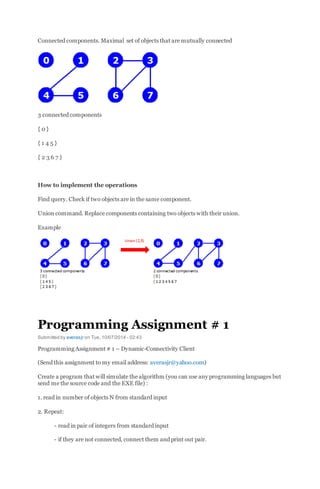
Program 1.1 is an implementation of a simple algorithm called the quick-find algorithm that
solves the connectivity problem (see Section 3.1 and Program 3.1 for basic information on Java
programs). The basis of this algorithm is an array of integers with the property that p and q are
connected if and only if the p th and q th array entries are equal. We initialize the i th array
entry to i for 0 i < N . To implement the unionoperation for p and q , we go through the

8. array, changing all the entries with the same name as p to have the same name as q . This
choice is arbitrary—we could have decided to change all the entries with the same name as q to
have the same name as p .
Figure 1.3 shows the changes to the array for the union operations in the example in Figure
1.1. To implement find , we just test the indicated array entries for equality—hence the
name quick find . Theunion operation, on the other hand, involves scanning through the whole
array for each input pair.
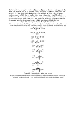
Figure 1.3. Example of quick find (slow union)
This sequence depicts the contents of the id array after each of the pairs at left is processed
by the quick-find algorithm ( Program 1.1 ). Shaded entries are those that change for the union
operation. When we process the pair pq , we change all entries with the value id[p] to have
the value id[q] .
Property 1.1
The quick-find algorithm executes at least MN instructions to solve a connectivity problem with
N objects that involves M union operations.
For each of the M union operations, we iterate the for loop N times. Each iteration requires at
least one instruction (if only to check whether the loop is finished).
We can execute tens or hundreds of millions of instructions per second on modern computers, so
this cost is not noticeable if M and N are small, but we also might find ourselves with billions of
objects and millions of input pairs to process in a modern application. The inescapable
conclusion is that we cannot feasibly solve such a problem using the quick-find algorithm (see
Exercise 1.10). We consider the process of precisely quantifying such a conclusion precisely in
Chapter 2.
Figure 1.4 shows a graphical representation of Figure 1.3. We may think of some of the objects
as representing the set to which they belong, and all of the other objects as having a link to the
representative in their set. The reason for moving to this graphical representation of the array will
become clear soon. Observe that the connections between objects (links) in this representation
are not necessarily the same as the connections in the input pairs—they are the information that
the algorithm chooses to remember to be able to know whether future pairs are connected.
Figure 1.4. Tree representation of quick find
This figure depicts graphical representations for the example in Figure 1.3 . The connections in these figures do
not necessarily represent the connections in the input. For example, the structure at the bottom has the
connection 1-7 , which is not in the input, but which is made because of the string of connections7-3-4-9-5-
6-1 .

9. The next algorithm that we consider is a complementary method called the quick-union algorithm . It
is based on the same data structure—an array indexed by object names—but it uses a different
interpretation of the values that leads to more complex abstract structures. Each object has a link
to another object in the same set, in a structure with no cycles. To determine whether two objects
are in the same set, we follow links for each until we reach an object that has a link to itself. The
objects are in the same set if and only if this process leads them to the same object. If they are
not in the same set, we wind up at different objects (which have links to themselves). To form
the union, then, we just link one to the other to perform the union operation; hence the name quick
union .
Figure 1.5 shows the graphical representation that corresponds to Figure 1.4 for the operation of
the quick-union algorithm on the example of Figure 1.1, and Figure 1.6 shows the corresponding
changes to the id array. The graphical representation of the data structure makes it relatively
easy to understand the operation of the algorithm—input pairs that are known to be connected in
the data are also connected to one another in the data structure. As mentioned previously, it is
important to note at the outset that the connections in the data structure are not necessarily the
same as the connections in the application implied by the input pairs; rather, they are constructed
by the algorithm to facilitate efficient implementation of union and find .
Figure 1.5. Tree representation of quick union
This figure is a graphical representation of the example in Figure 1.3 . We draw a line from object i to
object id[i] .

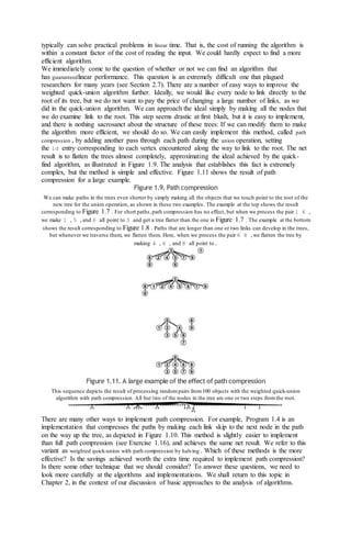
10. Figure 1.6. Example of quick union (not-too-quick find)
This sequence depicts the contents of the id array after each of the pairs at left are processed by the quick-union
algorithm ( Program 1.2 ). Shaded entries are those that change for the union operation (just one per operation).
When we process the pair p q , we follow links from p to get an entry i with id[i] == i ; then, we follow
links from q to get an entry j with id[j] == j ; then, if i and j differ, we set id[i] = id[j] . For the
find operation for the pair 5-8 (final line), i takes on the values 5 6901 , and j takes on the values 801 .
The connected components depicted in Figure 1.5 are called trees ; they are fundamental
combinatorial structures that we shall encounter on numerous occasions throughout the book.
We shall consider the properties of trees in detail in Chapter 5. For the union and find operations,
the trees in Figure 1.5 are useful because they are quick to build and have the property that two
objects are connected in the tree if and only if the objects are connected in the input. By moving
up the tree, we can easily find the root of the tree containing each object, so we have a way to
find whether or not they are connected. Each tree has precisely one object that has a link to itself,
which is called the root of the tree. The self-link is not shown in the diagrams. When we start at
any object in the tree, move to the object to which its link refers, then move to the object to

11. which that object's link refers, and so forth, we always eventually end up at the root. We can
prove this property to be true by induction: It is true after the array is initialized to have every
object link to itself, and if it is true before a given union operation, it is certainly true afterward.
The diagrams in Figure 1.4 for the quick-find algorithm have the same properties as those
described in the previous paragraph. The difference between the two is that we reach the root
from all the nodes in the quick-find trees after following just one link, whereas we might need to
follow several links to get to the root in a quick-union tree.
Program 1.2 Quick-union solution to connectivity problem
If we replace the body of the for loop in Program 1.1 by this code, we have a program that
meets the same specifications as Program 1.1, but does less computation for the union operation at
the expense of more computation for the find operation. The for loops and
subsequent if statement in this code specify the necessary and sufficient conditions on
the id array for p and q to be connected. The assignment statement id[i] = j implements
the union operation.
int i, j, p = In.getInt(), q = In.getInt(); for (i = p; i != id[i]; i = id[i ]); for (j =
q; j != id[j]; j = id[j]); if (i == j) continue; id[i] = j; Out.println(" " + p + " " +
q);
Program 1.2 is an implementation of the union and find operations that comprise the quick-union
algorithm to solve the connectivity problem. The quick-union algorithm would seem to be faster
than the quick-find algorithm, because it does not have to go through the entire array for each
input pair; but how much faster is it? This question is more difficult to answer here than it was
for quick find, because the running time is much more dependent on the nature of the input. By
running empirical studies or doing mathematical analysis (see Chapter 2), we can convince
ourselves that Program 1.2 is far more efficient than Program 1.1, and that it is feasible to
consider using Program 1.2 for huge practical problems. We shall discuss one such empirical
study at the end of this section. For the moment, we can regard quick union as an improvement
because it removes quick find's main liability (that the program requires at leastNM instructions
to process M union operations among N objects).
This difference between quick union and quick find certainly represents an improvement, but
quick union still has the liability that we cannot guarantee it to be substantially faster than quick
find in every case, because the input data could conspire to make the find operation slow.
Property 1.2
For M > N, the quick-union algorithm could take more than MN/ 2 instructions to solve a connectivity problem with
M pairs of N objects.
Suppose that the input pairs come in the order 1-2 , then 2-3 , then 3-4 , and so forth. After N -
1 such pairs, we have N objects all in the same set, and the tree that is formed by the quick-union
algorithm is a straight line, with N linking to N - 1, which links to N - 2, which links to N - 3, and
so forth. To execute the find operation for object N , the program has to follow N - 1 links. Thus,
the average number of links followed for the first N pairs is
Now suppose that the remainder of the pairs all connect N to some other object.
The find operation for each of these pairs involves at least ( N - 1) links. The grand total for the M
find operations for this sequence of input pairs is certainly greater than MN/ 2.
Fortunately, there is an easy modification to the algorithm that allows us to guarantee that bad
cases such as this one do not occur. Rather than arbitrarily connecting the second tree to the first
for union , we keep track of the number of nodes in each tree and always connect the smaller tree
to the larger. This change requires slightly more code and another array to hold the node counts,
as shown in Program 1.3, but it leads to substantial improvements in efficiency. We refer to this
algorithm as the weighted quick-union algorithm .
Figure 1.7 shows the forest of trees constructed by the weighted union-find algorithm for the
example input in Figure 1.1. Even for this small example, the paths in the trees are substantially

12. shorter than for the unweighted version in Figure 1.5. Figure 1.8 illustrates what happens in the
worst case, when the sizes of the sets to be merged in the union operation are always equal (and a
power of 2). These tree structures look complex, but they have the simple property that the
maximum number of links that we need to follow to get to the root in a tree of 2 n
nodes is n .
Furthermore, when we merge two trees of 2 n
nodes, we get a tree of 2 n +1
nodes, and we increase
the maximum distance to the root to n + 1. This observation generalizes to provide a proof that
the weighted algorithm is substantially more efficient than the unweighted algorithm.
Figure 1.7. Tree representation of weighted quick union
This sequence depicts the result of changing the quick-union algorithm to link the root of the smaller of the two trees
to the root of the larger of the two trees. The distance from each node to the root of its tree is small, so the find
operation is efficient.
Figure 1.8. Weighted quick union (worst case)
The worst scenario for the weighted quick-union algorithm is that each union operation links trees of equal size. If
the number of objects is less than 2 n
, the distance fromany node to the root of its tree is less than n .

13. Program 1.3 Weighted version of quick union
This program is a modification to the quick-union algorithm (see Program 1.2) that keeps an
additional array sz for the purpose of maintaining, for each object with id[i] == i , the
number of nodes in the associated tree so that the union operation can link the smaller of the two
specified trees to the larger, thus preventing the growth of long paths in the trees.
public class QuickUW { public static void main(String[] args) { int N =
Integer.parseInt(args[0]); int id[] = new int[N], sz[] = new int[N]; for (int i =
0;i<N;i++) { id[i] = i; sz[i] = 1; } for(In.init(); !In.empty(); ) { int i, j, p =
In.getInt(), q = In.getInt(); for (i = p; i != id[i]; i = id[i]); for (j = q; j != id[j];
j = id[j]); if (i == j) continue; if (sz[i] < sz[j]) { id[i] = j; sz[j] += sz[i]; }
else { id[j] = i; sz[i] += sz[j]; } Out.println(" " + p +""+q); } } }
Property 1.3
The weighted quick-union algorithm follows at most 2 lg N links to determine whether two of N objects are
connected.
We can prove that the union operation preserves the property that the number of links followed
from any node to the root in a set of k objects is no greater than lg k (we do not count the self-link
at the root). When we combine a set of i nodes with a set of j nodes with i j , we increase the
number of links that must be followed in the smaller set by 1, but they are now in a set of
size i + j , so the property is preserved because 1 + lg i =lg( i + i ) lg( i + j ).
The practical implication of Property 1.3 is that the weighted quick-union algorithm uses at most a
constant times M lg N instruc-tions to process M edges on N objects (see Exercise 1.9). This result
is in stark contrast to our finding that quick find always (and quick union sometimes) uses at least
MN/ 2 instructions. The conclusion is that, with weighted quick union, we can guarantee that we
can solve huge practical problems in a reasonable amount of time (see Exercise 1.11). For the
price of a few extra lines of code, we get a program that is literally millions of times faster than
the simpler algorithms for the huge problems that we might encounter in practical applications.
It is evident from the diagrams that relatively few nodes are far from the root; indeed, empirical
studies on huge problems tell us that the weighted quick-union algorithm of Program 1.3

14. typically can solve practical problems in linear time. That is, the cost of running the algorithm is
within a constant factor of the cost of reading the input. We could hardly expect to find a more
efficient algorithm.
We immediately come to the question of whether or not we can find an algorithm that
has guaranteedlinear performance. This question is an extremely difficult one that plagued
researchers for many years (see Section 2.7). There are a number of easy ways to improve the
weighted quick-union algorithm further. Ideally, we would like every node to link directly to the
root of its tree, but we do not want to pay the price of changing a large number of links, as we
did in the quick-union algorithm. We can approach the ideal simply by making all the nodes that
we do examine link to the root. This step seems drastic at first blush, but it is easy to implement,
and there is nothing sacrosanct about the structure of these trees: If we can modify them to make
the algorithm more efficient, we should do so. We can easily implement this method, called path
compression , by adding another pass through each path during the union operation, setting
the id entry corresponding to each vertex encountered along the way to link to the root. The net
result is to flatten the trees almost completely, approximating the ideal achieved by the quick-
find algorithm, as illustrated in Figure 1.9. The analysis that establishes this fact is extremely
complex, but the method is simple and effective. Figure 1.11 shows the result of path
compression for a large example.
Figure 1.9. Path compression
We can make paths in the trees even shorter by simply making all the objects that we touch point to the root of the
new tree for the union operation, as shown in these two examples. The example at the top shows the result
corresponding to Figure 1.7 . For short paths,path compression has no effect, but when we process the pair 1 6 ,
we make 1 , 5 , and 6 all point to 3 and get a tree flatter than the one in Figure 1.7 . The example at the bottom
shows the result corresponding to Figure 1.8 . Paths that are longer than one or two links can develop in the trees,
but whenever we traverse them, we flatten them. Here, when we process the pair 6 8 , we flatten the tree by
making 4 , 6 , and 8 all point to .
Figure 1.11. A large example of the effect of path compression
This sequence depicts the result of processing random pairs from100 objects with the weighted quick-union
algorithm with path compression. All but two of the nodes in the tree are one or two steps fromthe root.
There are many other ways to implement path compression. For example, Program 1.4 is an
implementation that compresses the paths by making each link skip to the next node in the path
on the way up the tree, as depicted in Figure 1.10. This method is slightly easier to implement
than full path compression (see Exercise 1.16), and achieves the same net result. We refer to this
variant as weighted quick-union with path compression by halving . Which of these methods is the more
effective? Is the savings achieved worth the extra time required to implement path compression?
Is there some other technique that we should consider? To answer these questions, we need to
look more carefully at the algorithms and implementations. We shall return to this topic in
Chapter 2, in the context of our discussion of basic approaches to the analysis of algorithms.

15. Figure 1.10. Path compression by halving
We can nearly halve the length of paths on the way up the tree by taking two links at a time and setting the bottom
one to point to the same node as the top one, as shown in this example. The net result of performing this operation
on every path that we traverse is asymptotically the same as full path compression.
Program 1.4 Path compression by halving
If we replace the for loops in Program 1.3 by this code, we halve the length of any path that we
traverse. The net result of this change is that the trees become almost completely flat after a long
sequence of operations.
for (i = p; i != id[i]; i = id[i]) id[i] = id[id[i]]; for (j = q; j != id[j]; j = id[j])
id[j] = id[id[j]];
The end result of the succession of algorithms that we have considered to solve the connectivity
problem is about the best that we could hope for in any practical sense. We have algorithms that
are easy to implement whose running time is guaranteed to be within a constant factor of the cost
of gathering the data. Moreover, the algorithms are online algorithms that consider each edge
once, using space proportional to the number of objects, so there is no limitation on the number
of edges that they can handle. The empirical studies in Table 1.1 validate our conclusion that
Program 1.3 and its path-compression variations are useful even for huge practical applications.
Choosing which is the best among these algorithms requires careful and sophisticated analysis
(see Chapter 2).
Exercises
1.4 Show the contents ofthe id array after each union operation when you use the quick-find algorithm
(Program 1.1) to solve the connectivity problem for the sequence 0-2 , 1-4 , 2-5 , 3-6 , 0-4 , 6-0 , and 1-
3. Also give the number of times the program accesses the id array for each input pair.
1.5 Do Exercise 1.4, but use the quick-union algorithm (Program 1.2).
Table 1.1. Empiricalstudy ofunion-find algorithms
These relative timings for solving random connectivity problems using various union-find algorithms
demonstrate the effectiveness of the weighted version of the quick-union algorithm. The added
incremental benefit due to path compression is less important. In these experiments, M is the number of
random connections generated until all N objects are connected.This process involves substantially
more find operations than union operations, so quick union is substantially slower than quick find.
Neither quick find nor quick union is feasible for huge N . The running time for the weighted methods is
evidently roughly proportional to M .
N M F U W P H
1000 3819 63 53 17 18 15
2500 12263 185 159 22 19 24
5000 21591 698 697 34 33 35

16. 10000 41140 2891 3987 85 101 74
25000 162748 237 267 267
50000 279279 447 533 473
100000 676113 1382 1238 1174
Key :
F quick find (Program 1.1)
U quick union (Program 1.2)
W weighted quick union (Program 1.3)
P weighted quick union with path compression (Exercise 1.16)
H weighted quick union with halving (Program 1.4)
1.6 Give the contents ofthe id array after each union operation for the weighted quick-union algorithm running
on the examples corresponding to Figure 1.7 and Figure 1.8.
1.7 Do Exercise 1.4, but use the weighted quick-union algorithm (Program 1.3).
1.8 Do Exercise 1.4, but use the weighted quick-union algorithm with path compression by halving (Program
1.4).
1.9 Prove an upper bound on the number of machine instructions required to process M connections on Nobjects
using Program 1.3. You may assume, for example, that any Java assignment statement always requires less
than c instructions,for some fixed constant c .
1.10 Estimate the minimum amount of time (in days)that would be required for quick find (Program 1.1) to solve a
problem with 10 9
objects and 10 6
input pairs, on a computer capable of executing 10 9
instructions per second.
Assume that each iteration of the inner for loop requires at least 10 instructions.
1.11 Estimate the maximum amount of time (in seconds)that would be required for weighted quick union (Program
1.3) to solve a problem with 10 9
objects and 10 6
input pairs, on a computer capable of executing 10 9
instructions per
second.Assume that each iteration of the outer for loop requires at most 100 instructions.
1.12 Compute the average distance from a node to the root in a worst-case tree of 2 n
nodes built by the weighted
quick-union algorithm.
1.13 Draw a diagram like Figure 1.10, starting with eight nodes instead of nine.
1.14 Give a sequence ofinput pairs that causes the weighted quick-union algorithm (Program 1.3) to produce a
path of length 4.
1.15 Give a sequence ofinput pairs that causes the weighted quick-union algorithm with path compression by
halving (Program 1.4) to produce a path of length 4.
1.16 Show how to modify Program 1.3 to implement full path compression, where we complete each unionoperation
by making every node that we touch link to the root of the new tree.
1.17 Answer Exercise 1.4, but use the weighted quick-union algorithm with full path compression (Exercise
1.16).
1.18 Give a sequence of input pairs that causes the weighted quick-union algorithm with full path
compression (Exercise 1.16) to produce a path of length 4.
1.19 Give an example showing that modifying quick union (Program 1.2) to implement full path compression
(see Exercise 1.16) is not sufficient to ensure that the trees have no long paths.
1.20 Modify Program 1.3 to use the height of the trees (longest path from any node to the root), instead of the
weight, to decide whether to set id[i] = j or id[j] = i . Run empirical studies to compare this variant with
Program 1.3.
1.21 Show that Property 1.3 holds for the algorithm described in Exercise 1.20.
1.22 Modify Program 1.4 to generate random pairs of integers between 0 and N - 1 instead of reading them from
standard input, and to loop until N - 1 union operations have been performed. Run your program for N = 10 3
,10 4
,
10 5
,and 10 6
,and print out the total number of edges generated for each value of N .
1.23 Modify your program from Exercise 1.22 to plot the number of edges needed to connect N items, for
100 N 1000.
1.24 Give an approximate formula for the number of random edges that are required to connect Nobjects, as
a function of N .

17. Lecture 3
Submitted by averasjr on Mon, 10/13/2014 - 09:01
Week 3 – Quick-Find
We’ll look at the first implementation of an algorithm for solving connectivity problem called
the Quick-Find. This is so called the EAGERALGORITHM or EAGER APPROACH.
The data structure that we are going to use to support the algorithm is simply an integer array
indexed by object.
 Integer array id[ ] of size N
The interpretation is the objects p and q are connected if-and-only-if their entries in the array are
the same.
 p and q are connected iff they have the same id
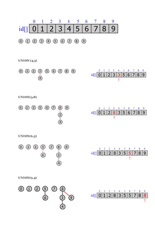
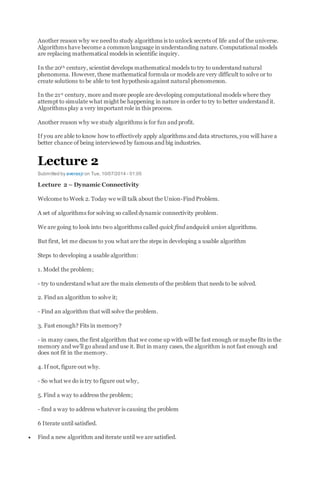
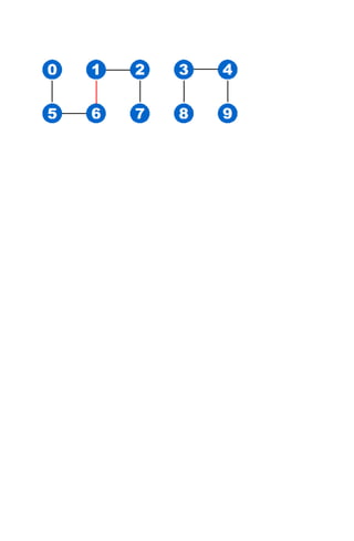
For example, the ten objects with id[ ] array describes the situation after 7 connections is
illustrated as follows:
At this point:
0, 5 and 6 are connected because they have the same id[ ] array zero (0).
1, 2 and 7 are connected because they have the same entry -> 1
1, 4, 8, and 9 are connected because they have the same entry -> 8
Thus the representation shows that these objects are connected as shown below:

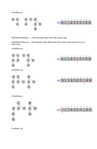
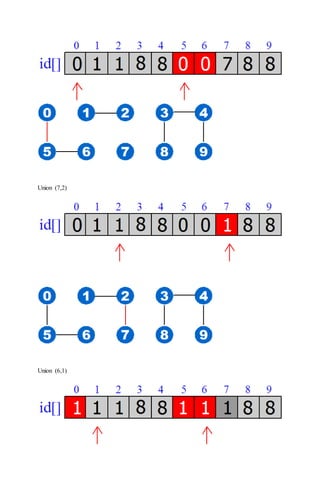
18. FIND: Check if p and q have the same id
id[6] = 0, id[1] = 1
6 and 1 are not connected
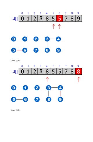
UNION: To merge components containing p and q, change all entries whose id equals id[p] to
id[q].
The entries were changed after:
Union (6,1)
The entries changed because from the original connected components, we connected 1 and 6:
Let’s have an example how this works:
Initially we set up the id[ ] array with each entry equal to its index as shown below:
Union (4,3)

19. we are going to change all entries whose id is equal to the first id to the second one. In this case,
we are going to change the id[4] = 3.
Union (3,8)
Union (6,5)

20. Union (9,4)
Union (2,1)

21. Connected(8,9) – Yes, they are already connected because they have the same id[ ] array. It
would return TRUE
Connected(5,0) – No, they are not connected because they have different id[ ] array. It would
return FALSE.
Union (5,0)

22. Union (7,2)
Union (6,1)

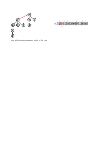
24. Lecture 4 – Quick-Union (Lazy Approach)
Another alternative to quick-union algorithm is the lazy approach.
It uses the same data structure with an integer array of size N:
 Integer array id[ ] of size N
But it has a different interpretation. We are going to think of that array as representing a set
of trees. Each entry in the array is going to contain a reference to its parent in a tree.
 Interpretation: id[ ] is parent of i.
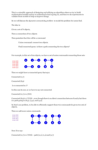
For example:
3’s parent is 4;
4’s parent is 9;
So 3’s entry is 4 and 4’s entry is 9.
 Root of I is id[ id[ id[…id[i]…]]]
Each entry in the array has associated with it a root, that’s a root of its tree. Elements that
are all by themselves with their own connected components points to themselves. Like 9 not
only points to itself but it is also connected to 2, 4, and 3 making 9 the root of these
components.
From this data structure we can associate with each item a root which is a representative of
its connected components.

25. Once we can calculate this roots then we can implement the FIND operation just by
checking whether the two items have the same root. That is equivalent to saying “are they in
the same connected component?”
 FIND. Check if p and q have the same root.
On the other hand, the UNION operation is very easy. To merge components containing two
different items that is in different components. All we do is set the id of p’s root to the id of
q’s root. That makes p’s root point to q. So in this case, we change the entry of 9 to be 6 to
merge 3 and 5 and we will change just one value in the array.
 UNION. To merge components containing p and q, set the id of p’s root to the id of q’s root.
That’s the quick-union algorithm because the union operation only involves changing one
entry in the array. Find operation requires a little more work.
An Implementation of the Quick – Union algorithm
We will assign values to the array id[ ] just like what we did in our previous
implementations of algorithm.

26. UNION (4,3)
UNION(3,8)
UNION(6,5)
UNION(9,4)

27. UNION(2,1)
CONNECTED(8,9) -> YES, because they have the same root
CONNECTED(5,4) -> NO, because they don’t have the same root (5 root is 5 & 4
root is 8).
UNION(5,0)
UNION(7,2)
UNION(6,1)
UNION(7,3)

28. Now we have one component with 8 as the root.