Ha2512781284

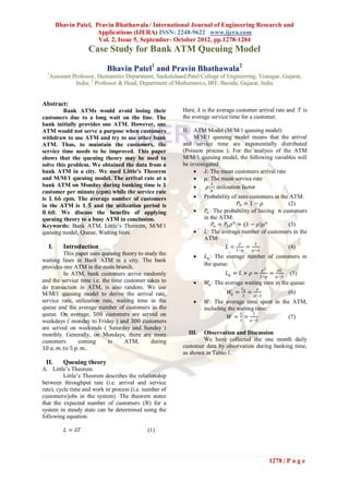
Bhavin Patel, Pravin Bhathawala / International Journal of Engineering Research and
Applications (IJERA) ISSN: 2248-9622 www.ijera.com
Vol. 2, Issue 5, September- October 2012, pp.1278-1284
Case Study for Bank ATM Queuing Model

Bhavin Patel1 and Pravin Bhathawala2
1
Assistant Professor, Humanities Department, Sankalchand Patel College of Engineering, Visnagar, Gujarat,
India; 2 Professor & Head, Department of Mathematics, BIT, Baroda, Gujarat, India

Abstract:
Bank ATMs would avoid losing their Here, 𝜆 is the average customer arrival rate and 𝑇 is
customers due to a long wait on the line. The the average service time for a customer.
bank initially provides one ATM. However, one
ATM would not serve a purpose when customers B. ATM Model (M/M/1 queuing model)
withdraw to use ATM and try to use other bank M/M/1 queuing model means that the arrival
ATM. Thus, to maintain the customers, the and service time are exponentially distributed
service time needs to be improved. This paper (Poisson process ). For the analysis of the ATM
shows that the queuing theory may be used to M/M/1 queuing model, the following variables will
solve this problem. We obtained the data from a be investigated:
bank ATM in a city. We used Little’s Theorem  𝜆: The mean customers arrival rate
and M/M/1 queuing model. The arrival rate at a  𝜇: The mean service rate
bank ATM on Monday during banking time is 𝟏 𝜆
 𝜌: 𝜇 : utilization factor
customer per minute (cpm) while the service rate
is 𝟏. 𝟔𝟔 cpm. The average number of customers  Probability of zero customers in the ATM:
in the ATM is 𝟏. 𝟓 and the utilization period is 𝑃0 = 1 − 𝜌 (2)
𝟎. 𝟔𝟎. We discuss the benefits of applying  𝑃𝑛 : The probability of having 𝑛 customers
queuing theory to a busy ATM in conclusion. in the ATM:
Keywords: Bank ATM, Little’s Theorem, M/M/1 𝑃𝑛 = 𝑃0 𝜌 𝑛 = (1 − 𝜌)𝜌 𝑛 (3)
queuing model, Queue, Waiting lines  𝐿: The average number of customers in the
ATM:
𝜌 𝜆
I. Introduction 𝐿 = 1−𝜌 = 𝜇 −𝜆 (4)
This paper uses queuing theory to study the
 𝐿 𝑞 : The average number of customers in
waiting lines in Bank ATM in a city. The bank
the queue:
provides one ATM in the main branch. 𝜌2 𝜌𝜆
In ATM, bank customers arrive randomly 𝐿 𝑞 = 𝐿 × 𝜌 = 1−𝜌 = (5)
𝜇 −𝜆
and the service time i.e. the time customer takes to  𝑊𝑞 : The average waiting time in the queue:
do transaction in ATM, is also random. We use 𝐿𝑞 𝜌
M/M/1 queuing model to derive the arrival rate, 𝑊𝑞 = = (6)
𝜆 𝜇 −𝜆
service rate, utilization rate, waiting time in the  𝑊: The average time spent in the ATM,
queue and the average number of customers in the including the waiting time:
queue. On average, 500 customers are served on 𝑊= =
𝐿 1
(7)
weekdays ( monday to Friday ) and 300 customers 𝜆 𝜇 −𝜆
are served on weekends ( Saturday and Sunday )
monthly. Generally, on Mondays, there are more III. Observation and Discussion
customers coming to ATM, during We have collected the one month daily
10 𝑎. 𝑚. 𝑡𝑜 5 𝑝. 𝑚.. customer data by observation during banking time,
as shown in Table-1.
II. Queuing theory
A. Little’s Theorem
Little’s Theorem describes the relationship
between throughput rate (i.e. arrival and service
rate), cycle time and work in process (i.e. number of
customers/jobs in the system). The theorem states
that the expected number of customers (𝑁) for a
system in steady state can be determined using the
following equation:

𝐿 = 𝜆𝑇 (1)

1278 | P a g e

Table-1 Monthly Customer counts
Sun Mon Tue Wed Thu Fri Sat
st
1 week 70 139 128 116 119 112 138
2nd week 71 155 140 108 72 78 75
3rd week 70 110 111 83 94 119 113
4th week 40 96 90 87 70 60 70
Total 251 500 469 394 355 369 396

180
160
140
120
1st week
100
2nd week
80
3rd week
60
4th week
40
20
0
1 2 3 4 5 6 7

Figure-1 one month daily customer counts

600

500

400

300

200

100

0
1 2 3 4 5 6 7

Figure-2 one month total customer counts

1279 | P a g e

From the above figure-1, we can say that, The queuing theory provides the formula to
the number of customers on Mondays is double the calculate the probability of having 𝑛 customers in
number of customers on Sundays during a month. the ATM as follows:
The busiest period for the bank ATM is on Mondays
and Tuesdays during banking time 𝑃𝑛 = 1 − 𝜌 𝜌 𝑛 = 1 − 0.60 (0.60) 𝑛 = (0.40)(0.60) 𝑛
(10 𝑎. 𝑚. 𝑡𝑜 5 𝑝. 𝑚.). Hence, we will focus our
analysis in this time period. Also, we can observe We assume that impatient customers will
from figure-2 that, after Monday, the number of start to balk when they see more than 3 people are
customers start decreasing slowly as the week already queuing for the ATM. We also assume that
progresses. On Thursdays, it is least and on Fridays the maximum queue length that a patient customer
and Saturdays, it stays slightly more than Thursdays. can tolerate is 10 people. As the capacity of the
This is because the next day will be a holiday. ATM is 1 people, we can calculate the probability
of 4 people in the system (i.e in the ATM).
A. Calculation Therefore, the probability of customers going away
We have observed that, after Sunday, = 𝑃(more than 3 people in the queue) = 𝑃(more
during first two days of a week, there are, on than 4 people in the ATM) is
average 60 people coming to the ATM in one hour 11
time period of banking time. From this we can 𝑃5−11 = 𝑃𝑛 = 0.07558 = 7.55 %
derive the arrival rate as: 𝑛=5

B. Evaluation
60  The utilization is directly proportional with
  1 customer/minute (cpm)
60 the mean number of customers. It means that
the mean number of customers will increase
We also found out from observation that as the utilization increases.
each customer spends 3/2 minutes on average in the  The utilization rate at the ATM is at 0.60.
ATM (𝑊), the queue length is around 1 people (𝐿 𝑞 ) However, this is the utilization rate during
on average and the average waiting time is around banking time on Mondays and Tuesdays. On
1/2 minutes i.e. 30 seconds. weekend, the utilization rate is almost half of
Theoretically, the average waiting time is it. This is because the number of people on
weekends is only half of the number of
𝐿𝑞 1 𝑐𝑢𝑠𝑡𝑜𝑚𝑒𝑟
𝑊𝑞 = = = 1 𝑚𝑖𝑛𝑢𝑡𝑒 people on weekdays.
𝜆 1 𝑐𝑝𝑚
 In case of the customers waiting time is lower
From this calculation, we can see that, the or in other words, we waited for less than 30
observed actual waiting time does not differ by seconds, the number of customers that are
much when it is compared with the theoretical able to be served per minute will increase.
waiting time. When the service rate is higher the utilization
Next, we will calculate the average number will be lower, which makes the probability of
of people in the ATM using (1), the customers going away decreases.
3 3 C. Benefits
𝐿 = 1 𝑐𝑝𝑚 × 𝑚𝑖𝑛𝑢𝑡𝑒𝑠 = = 1.5 𝑐𝑢𝑠𝑡𝑜𝑚𝑒𝑟𝑠
2 2
 This research can help bank ATM to increase
Using (4), we can also derive the utilization rate and its QoS (Quality of Service), by anticipating,
the service rate. if there are many customers in the queue.
3  The result of this paper is helpful to analyse
𝜆(1 + 𝐿) 1(1 + 2) 5/2 5 the current system and improve the next
𝜇= = = = = 1.66 𝑐𝑝𝑚
𝐿 3 3/2 3 system. Because the bank can now estimate
2 the number of customers waiting in the queue
𝜆 1 𝑐𝑝𝑚 3
Hence, 𝜌 = 𝜇 = 5 = 5 = 0.60 and the number of customers going away
𝑐𝑝𝑚
3 each day.
 By estimating the number of customers
This is the probability that, the server, in
coming and going in a day, the bank can set a
this case ATM, is busy to serve the customers,
target that, how many ATMs are required to
during banking time. So, during banking time, the
serve people in the main branch or any other
probability of zero customers in the ATM is
branch of the bank.
𝑃0 = 1 − 𝜌 = 1 − 0.60 = 0.40
IV. Conclusion
This paper has discussed the application of
queuing theory to the Bank ATM. From the result,

1280 | P a g e

we have obtained that, the rate at which customers other branch ATM also. In this way, this research
arrive in the queuing system is 1 customer per can contribute to the betterment of a bank in terms
minute and the service rate is 1.66 customers per of its functioning through ATM.
minute. The probability of buffer flow if there are 3 Now, we will develop a simulation model
or more customers in the queue is 7 out of 100 for the ATM. By developing a simulation model, we
customers. The probability of buffer overflow is the will be able to confirm the results of the analytical
probability that, customers will run away, because model that we develop in this paper. By this model,
may be they are impatient to wait in the queue. This it can mirror the actual operation of the ATM more
theory is also applicable for the bank, if they want to closely.
calculate all the data daily and this can be applied to

We discuss the simulation of ATM model as follows:

Simulation of a Single-Server Queuing Model

Nbr of arrivals = 125 <<Maximum 500
Enter x in column A to select interarrival pdf:
Constant =

x Exponential: 1
Uniform: a= b=
Triangular: a= b= c=
Enter x in column A to select service time pdf:
Constant =

Exponential: 1.66
x Uniform: a= 0.5
b= 0.8
Triangular: a= b= c=
Output Summary
Av. facility utilization = 0.63
Percent idleness (%) = 36.82

Av. queue length, Lq = 0.44
Av. nbr in system, Ls = 1.07 Press F9 to
Av. queue time, Wq = 0.46 trigger a
Av. system time, Ws = 1.13 new simulation
run.
Sum(ServiceTime) = 83.49
Sum(Wq) = 57.58
Sum(Ws) = 141.07

Nbr InterArvlTime ServiceTime ArrvlTime DepartTime Wq Ws
1 1.79 0.55 0.00 0.55 0.00 0.55
2 0.68 0.56 1.79 2.35 0.00 0.56
3 0.51 0.79 2.47 3.26 0.00 0.79
4 1.05 0.70 2.98 3.96 0.28 0.98
5 0.90 0.61 4.03 4.64 0.00 0.61
6 1.42 0.57 4.93 5.50 0.00 0.57
7 0.58 0.63 6.35 6.98 0.00 0.63
8 0.68 0.74 6.93 7.72 0.05 0.79
9 0.42 0.60 7.61 8.32 0.11 0.71
10 2.76 0.52 8.03 8.84 0.29 0.81
11 0.57 0.54 10.79 11.33 0.00 0.54
12 0.93 0.62 11.36 11.98 0.00 0.62

1281 | P a g e


13 0.30 0.54 12.29 12.83 0.00 0.54
14 1.29 0.51 12.59 13.34 0.24 0.75
15 0.44 0.78 13.88 14.66 0.00 0.78
16 1.32 0.53 14.32 15.19 0.34 0.87
17 0.43 0.63 15.64 16.27 0.00 0.63
18 0.64 0.65 16.07 16.92 0.20 0.85
19 1.15 0.72 16.71 17.64 0.21 0.93
20 0.34 0.76 17.86 18.62 0.00 0.76
21 0.94 0.62 18.20 19.24 0.42 1.04
22 1.28 0.74 19.14 19.98 0.10 0.84
23 3.65 0.75 20.42 21.17 0.00 0.75
24 1.08 0.78 24.07 24.85 0.00 0.78
25 2.60 0.68 25.15 25.83 0.00 0.68
26 2.16 0.65 27.75 28.40 0.00 0.65
27 1.90 0.64 29.91 30.55 0.00 0.64
28 0.81 0.64 31.81 32.45 0.00 0.64
29 2.08 0.63 32.62 33.25 0.00 0.63
30 1.63 0.78 34.70 35.48 0.00 0.78
31 0.31 0.57 36.33 36.90 0.00 0.57
32 0.74 0.71 36.64 37.61 0.26 0.97
33 2.00 0.70 37.38 38.31 0.23 0.93
34 0.31 0.61 39.38 39.99 0.00 0.61
35 0.12 0.66 39.69 40.65 0.30 0.96
36 1.91 0.60 39.81 41.25 0.84 1.44
37 0.00 0.55 41.72 42.27 0.00 0.55
38 1.27 0.67 41.72 42.94 0.55 1.22
39 0.67 0.71 42.99 43.70 0.00 0.71
40 0.51 0.76 43.66 44.46 0.04 0.80
41 0.02 0.70 44.17 45.16 0.29 0.99
42 0.08 0.55 44.19 45.71 0.97 1.52
43 0.42 0.76 44.27 46.47 1.44 2.20
44 1.88 0.69 44.69 47.16 1.78 2.47
45 0.12 0.76 46.57 47.92 0.59 1.35
46 3.54 0.69 46.69 48.61 1.23 1.92
47 1.11 0.66 50.23 50.89 0.00 0.66
48 1.02 0.78 51.34 52.12 0.00 0.78
49 0.57 0.63 52.36 52.99 0.00 0.63
50 0.69 0.70 52.93 53.69 0.06 0.76
51 2.19 0.68 53.62 54.37 0.07 0.75
52 0.18 0.59 55.81 56.40 0.00 0.59
53 0.46 0.57 55.99 56.97 0.41 0.98
54 0.08 0.78 56.45 57.75 0.52 1.30
55 1.60 0.74 56.53 58.49 1.22 1.96
56 0.55 0.57 58.13 59.06 0.36 0.93
57 0.80 0.75 58.68 59.81 0.38 1.13
58 0.22 0.55 59.48 60.36 0.33 0.88
59 1.76 0.72 59.70 61.08 0.66 1.38
60 0.72 0.72 61.46 62.18 0.00 0.72
61 1.15 0.58 62.18 62.76 0.00 0.58
62 4.52 0.59 63.33 63.92 0.00 0.59
63 2.04 0.71 67.85 68.56 0.00 0.71

1282 | P a g e

64 0.63 0.72 69.89 70.61 0.00 0.72
65 0.12 0.77 70.52 71.38 0.09 0.86
66 0.74 0.55 70.64 71.93 0.74 1.29
67 0.14 0.65 71.38 72.58 0.55 1.20
68 0.40 0.70 71.52 73.28 1.06 1.76
69 0.31 0.65 71.92 73.93 1.36 2.01
70 0.30 0.70 72.23 74.63 1.70 2.40
71 0.55 0.70 72.53 75.33 2.10 2.80
72 0.20 0.52 73.08 75.85 2.25 2.77
73 1.43 0.74 73.28 76.59 2.57 3.31
74 0.95 0.57 74.71 77.16 1.88 2.45
75 1.05 0.61 75.66 77.77 1.50 2.11
76 2.47 0.67 76.71 78.44 1.06 1.73
77 0.28 0.56 79.18 79.74 0.00 0.56
78 1.35 0.78 79.46 80.52 0.28 1.06
79 1.14 0.76 80.81 81.57 0.00 0.76
80 4.62 0.56 81.95 82.51 0.00 0.56
81 0.05 0.71 86.57 87.28 0.00 0.71
82 0.02 0.63 86.62 87.91 0.66 1.29
83 0.22 0.72 86.64 88.63 1.27 1.99
84 0.47 0.70 86.86 89.33 1.77 2.47
85 0.52 0.71 87.33 90.04 2.00 2.71
86 1.05 0.57 87.85 90.61 2.19 2.76
87 0.28 0.50 88.90 91.11 1.71 2.21
88 3.08 0.54 89.18 91.65 1.93 2.47
89 1.10 0.70 92.26 92.96 0.00 0.70
90 0.49 0.71 93.36 94.07 0.00 0.71
91 3.37 0.59 93.85 94.66 0.22 0.81
92 0.40 0.68 97.22 97.90 0.00 0.68
93 2.77 0.64 97.62 98.54 0.28 0.92
94 0.00 0.71 100.39 101.10 0.00 0.71
95 0.83 0.77 100.39 101.87 0.71 1.48
96 1.05 0.65 101.22 102.52 0.65 1.30
97 0.13 0.68 102.27 103.20 0.25 0.93
98 0.14 0.52 102.40 103.72 0.80 1.32
99 1.45 0.80 102.54 104.52 1.18 1.98
100 0.52 0.78 103.99 105.30 0.53 1.31
101 1.34 0.65 104.51 105.95 0.79 1.44
102 2.19 0.78 105.85 106.73 0.10 0.88
103 0.84 0.57 108.04 108.61 0.00 0.57
104 2.18 0.66 108.88 109.54 0.00 0.66
105 2.63 0.75 111.06 111.81 0.00 0.75
106 0.17 0.78 113.69 114.47 0.00 0.78
107 2.02 0.76 113.86 115.23 0.61 1.37
108 1.16 0.74 115.88 116.62 0.00 0.74
109 0.66 0.68 117.04 117.72 0.00 0.68
110 0.55 0.63 117.70 118.35 0.02 0.65
111 0.51 0.67 118.25 119.02 0.10 0.77
112 0.43 0.63 118.76 119.65 0.26 0.89
113 1.27 0.77 119.19 120.42 0.46 1.23
114 0.54 0.75 120.46 121.21 0.00 0.75
115 0.08 0.77 121.00 121.98 0.21 0.98
116 0.54 0.74 121.08 122.72 0.90 1.64
117 1.36 0.73 121.62 123.45 1.10 1.83

1283 | P a g e

118 4.13 0.62 122.98 124.07 0.47 1.09
119 0.81 0.73 127.11 127.84 0.00 0.73
120 0.64 0.55 127.92 128.47 0.00 0.55
121 0.00 0.77 128.56 129.33 0.00 0.77
122 0.03 0.73 128.56 130.06 0.77 1.50
123 0.31 0.53 128.59 130.59 1.47 2.00
124 1.86 0.74 128.90 131.33 1.69 2.43
125 0.01 0.77 130.76 132.10 0.57 1.34

By the simulation model, we can say that, (2) J.D.C. Little, “A Proof for the Queuing
the sum of the service time for 125 customers is Formula: 𝐿 = 𝜆𝑊”, Operations
83.48 minutes. Hence, the service time for one Research, vol. 9(3), 1961, pp. 383-387,
customer is 0.67 minutes. doi:10.2307/167570.
Therefore, the service rate 𝜇 =
1
= 1.49 𝑐𝑝𝑚. (3) K. Rust, “Using Little’s Law to
0.67 Estimate Cycle Time and Cost”,
The actual service rate is 𝜇 = 1.66 𝑐𝑝𝑚.
Proceedings of the 2008 Winter
So, we can say that, there is no much difference
Simulation Conference, IEEE Press,
between the actual service rate and the estimated
Dec. 2008,
service rate.
doi:10.1109/WSC.2008.4736323.
(4) H.A. Taha, Operations Research-An
References Introduction. 8th Edition, ISBN
(1) T. Altiok and B. Melamed, Simulation 0131889230. Pearson Education, 2007.
Modeling and Analysis with ARENA. (5) M. Laguna and J. Marklund, Business
ISBN 0-12-370523-1. Academic Press, Process Modeling, Simulation and
2007. Design. ISBN 0-13-091519-X. Pearson
Prentice Hall, 2005.

1284 | P a g e

Ha2512781284

Recommended

Recommended

More Related Content

Viewers also liked

Viewers also liked (20)

Similar to Ha2512781284

Similar to Ha2512781284 (20)

Ha2512781284