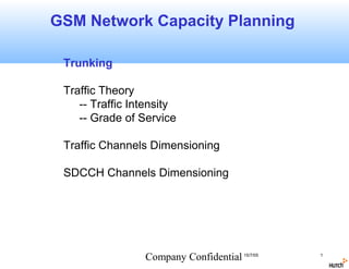
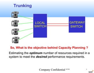
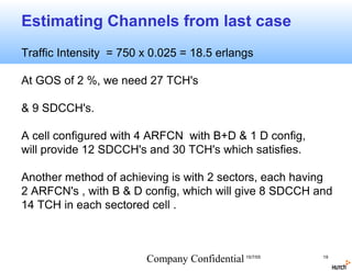
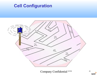
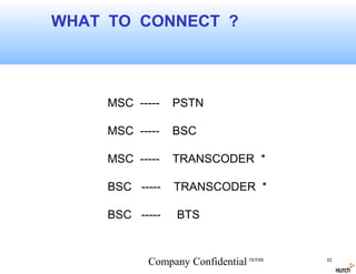
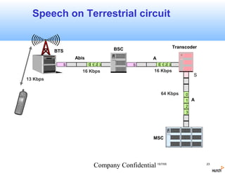
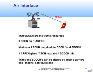
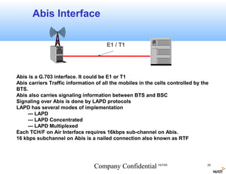
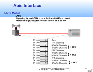
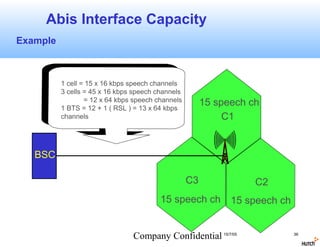
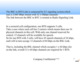
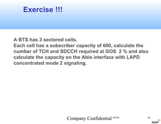
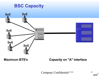
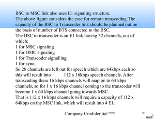
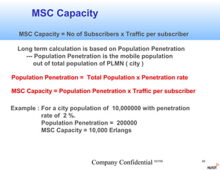
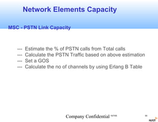
This document discusses capacity planning for GSM networks. It covers topics like trunking, traffic theory including traffic intensity, grade of service, busy hour, and request rate. It describes how to dimension traffic channels and SDCCH channels based on factors like traffic intensity and grade of service. It also discusses connectivity planning between network elements like MSC, BSC, transcoder, and BTS. It provides details on air interface, Abis interface between BSC and BTS, and different LAPD modes for signaling concentration over Abis. The objective is to estimate the optimal number of resources needed to meet performance requirements based on traffic analysis and engineering principles.
Call Setup Success Rate Definition and Troubleshooting Assim Mubder
The CSSR indicates the probability of successful calls initiated by the MS. The CSSR is an important KPI for evaluating the network performance. If this KPI is too low, the subscribers are not likely to make calls successfully. The user experience is thus affected.
Hello my friends
Unfortunately, if you want any of these files, please contact me by email and mention any reference you find, to give it to you.
My email: molham.shoriss@outlook.com
LTE
LTE Introduction
LTE Fundamental
LTE RNP Introduction
LTE Principles (Huawei eRAN 3.0)
LTE Access Fault Diagnosis
LTE Access Transport Network Dimensioning
LTE Air Interface ISSUE 1.05
LTE Cell Planning ISSUE1.10
LTE eRAN 3.0 Scheduling - Feature Parameter Description
LTE eRAN3.0 Idle Mode Behavior
LTE eRAN3.0 KPI Introduction
LTE eRAN3.0 - Mobility Management in Connected Mode - Feature Parameters Description
LTE Handover Fault Diagnosis
LTE Network Tuning ISSUE 1.00
LTE Protocols and Procedure
LTE Radio Network Capacity Dimensioning
LTE Radio Network Coverage Dimensioning
LTE Radio Resource Management Overview
LTE Scheduling
LTE (Eicsson)
01.LTE SAE System Overview
LTE 10A Air Interface
LTE L10A Access Transport Network
LTE L10A Radio Network Design
LTE L12 Initial Tuning
LTE L14 Radio Network Functionality LTE
LTE Protocols and Procedures
LTE System Techniques
LTE Throughput Troubleshooting Techniques
LTE Radio Access Radio Interface Dimensioning and Planning
MIMO in WCDMA and LTE
LTE L14 Radio Network Functionality LTE
LTE Huawei
LTE System Overview
LTE Air Interface
LTE Protocols and Signaling Procedures
LTE Network Performance Management (KPIs)
LTE Radio Network Coverage Dimensioning
LTE Cell Planning
LTE Access Fault Diagnosis
LTE Handover Fault Diagnosis
LTE Call Drop Diagnosis
LTE Traffic Fault Diagnosis
LTE Interference Troubleshooting Guide
LTE Optimization
LTE Troubleshooting Access Failures
Features 1. Idle Mode
Features 2. Intra Rat Handover
Features 3. Power Control
Features 4. Scheduling
Features 5. CS Fallback
Features 6. Physical Channel Resource Management
HedEx for LTE
eRAN_eRAN13.0_02_en_GEG09124
5G
5G System Design (Wiley)
HedEx for 5G
(For Engineer) 5G RAN2.0 Solution Technical Guideline
Hello my friends
Unfortunately, if you want any of these files, please contact me by email and mention any reference you find, to give it to you.
My email: molham.shoriss@outlook.com
In this paper, we discussed about LTE system throughput calculation for both TDD and FDD system.
3GPP LTE technology support both TDD and FDD multiplexing. The paper describes all the factors which affect the throughput like Bandwidth, Modulation, UE category and mulplexing. It also describes how we get throughput 300Mbps in DL and 75Mbps in UL and what are assumptions taken to calculate the same.
Paper describes the steps and formulae to calculate the throughput for FDD system for TDD Config 1 and Config 2.
The throughput calculations shown in this paper is theoretical and limited by the assumptions taken to calculate for calculations
In many countries, cities are expanding in terms of size, number residents and visitors, etc. The resulting increase in concentration of people, with their mobility needs, causes major traffic and transportation problems in and around our cities. Next to the economic impacts due to delay and unreliability of travel time, concerns regarding safety and security, emissions and sustainability become more and more urgent.
ITS (Intelligent Transportation Systems) hold the potential to reduce these issues. In the past decade, we have been more and more successful in making better use of the available infrastructure by using traditional ITS measures. As we will show in this talk, key to this success has been in achieving a profound understanding of what are the key phenomena that characterise network traffic flows, and designing solutions that capitalise on this.
The playing field is however rapidly changing. For one, we see a transition from road-side to in-car technology in terms of sensing and actuation. This provides great opportunities, but making best use of these is not trivial and requires a paradigm shift in the way we think about managing traffic flows where collaboration between the old stakeholders (e.g. road authorities) and the new stakeholders (e.g. companies like Google, and TomTom) becomes increasingly important. This will be illustrated in this talk by some examples showing how we can put the transition to in-car traffic management to use, both in terms of making optimal use of the new data sources and the use of the car as an actuator.
With respect to the latter, we will see that even for low penetration levels, which will occur in the transition phase towards a more highly automated traffic stream, considerable impacts can be achieved if we adequately consider the non-automated vehicles. Furthermore, it requires vehicles to be able to communicate and cooperate with each other.
These two elements are two of the five steps that was identified in the transition towards a fully automated system.
The final part of the talk will deal with the other steps that are deemed important to understand which of the scenarios in a urban self-driving future will unfold. These pertain to the interaction between man and machine, the need and willingness to invest in separate infrastructure in city, and whether automated car can co-exist with other (active) travel modes. With respect to the latter, we will also consider what ITS can mean for the other modes of travel.
NetWork Design Question2.) How does TCP prevent Congestion Dicuss.pdfoptokunal1
NetWork Design Question
2.) How does TCP prevent Congestion? Dicuss the information identifying congestion in the
network as well as the mechanism for reducing congestion?
Solution
Congestion is a problem that occurs on shared networks when multiple users contend for access
to the same resources (bandwidth, buffers, and queues).
Transmission Control Protocol (TCP) uses a network congestion-avoidance algorithm that
includes various aspects of an additive increase/multiplicative decrease (AIMD) scheme, with
other schemes such as slow-start to achieve congestion avoidance.
The TCP congestion-avoidance algorithm is the primary basis for congestion control in the
Internet.
Congestion typically occurs where multiple links feed into a single link, such as where internal
LANs are connected to WAN links. Congestion also occurs at routers in core networks where
nodes are subjected to more traffic than they are designed to handle.
TCP/IP networks such as the Internet are especially susceptible to congestion because of their
basic connection- less nature. There are no virtual circuits with guaranteed bandwidth. Packets
are injected by any host at any time, and those packets are variable in size, which make
predicting traffic patterns and providing guaranteed service impossible. While connectionless
networks have advantages, quality of service is not one of them.
Shared LANs such as Ethernet have their own congestion control mechanisms in the form of
access controls that prevent multiple nodes from transmitting at the same time.
Identifying:
Congestion is primarily reflected by a conventional user feeling-- slowness. This statement
reflects the change in the network effective flow, that is the time required to transmit an entire
data from one point to another. The effective flow doenot exist as such, it consists in reality of
three seperate indicators:
*Latency:the effective flow is inversely proportional to the latency.
*Jitter:it is latency variation over time, impacts by influencing the flow latency
*Loss Rate:the theoritical bandwidth is inversely proportional to the square root of the loss rate
These Congestion symtoms allow us to rely on objective indicators to characterize it.
Mechanism to reduce congestion:
The standard fare in TCP implementations today has four standard congestion control algorithms
that are now in common use. Their usefulness has passed the test of time.
The four algorithms, Slow Start, Congestion Avoidance, Fast Retransmit and Fast Recovery are
described below. (a) Slow Start
Slow Start, a requirement for TCP software implementations is a mechanism used by the sender
to control the transmission rate, otherwise known as sender-based flow control. This is
accomplished through the return rate of acknowledgements from the receiver. In other words, the
rate of acknowledgements returned by the receiver determine the rate at which the sender can
transmit data. When a TCP connection first begins, the Slow Start algorithm initializes a
.
USE TORA TODetermine the maximum flow and the optimum flow in eac.pdfseamusschwaabl99557
USE TORA TO:
Determine the maximum flow and the optimum flow in each arc for the network in the following
figure.
Clearly show all steps and data input.
Exterior Graph Data, Nodes listed outside paranthesis
Node 1 (14) to Node 3 (0)
Node 3 (10) to Node 5 (0)
Node 5(0) to Node 4 (5)
Node 4(6) to Node 2 (7)
Node 2(0) to Node 1 (8)
Interior Graph (Triangle ) Data
Node3 (10) to Node2(5)
Node3 (9) to Node 4(7)
Second Interior Graph Data
Node5 (0) to Node2(6)
Solution
The most successful and simple model is Erlang\'s loss system where the blocking probability is
given by Erlang\'s B-formula. The traffic is described by the offered traffic A, the system (only
one link) by the number of channels, and the strategy is full accessibility with lost calls cleared.
The above-mentioned three elements of the model are each described by only one parameter.
Only single-channel calls are considered. The network performance is described by the blocking
probability E1,n(A), i.e. the probability that a call attempts is blocked because all n channels are
busy. For Erlang\'s loss system time, call, and traffic congestions are equal. The state
probabilities are given by the truncated Poisson distribution, and when the number of channels is
very large this becomes a Poisson distribution. This model has been very successful for traffic
engineering. The background for this success is that the traffic is very well modeled by one
parameter only. The underlying mathematical assumption is a Poisson arrival process. This is
fulfilled when the traffic is generated by many independent users, which is the case for
telephony. If the arrival process is a Poisson process, then the model is insensitive to the holding
time distribution, which means that only the mean holding time is of importance. So the model is
very robust to the traffic and models the real world extremely well. Improvement function: This
denotes the increase in carried traffic when the number of channels is increased by one from n to
n + 1: 64 Attention: This is not an ITU publication made available to the public, but an internal
ITU Document intended only for use by the Member States of the ITU and by its Sector
Members and their respective staff and collaborators in their ITU related work. It shall not be
made available to, and used by, any other persons or entities without the prior written consent of
the ITU. ITU Telecom Network Planning Reference Manual - Draft version 4.1 January 2007
4.8.4.3 Engset\'s loss system The Poisson arrival process is the most random process, and the
calls are generated by a very large number of independent sources, each having an infinitesimal
calling rate. In many real systems the number of users is limited, and the arrival process is more
regular or smooth than random traffic. This is modeled by Engset\'s loss system where we have a
finite number S of users (traffic sources) which alternates between the states off (= idle) and on
(= busy). When a source is idle it generates cal.
Cellular wireless systems like GSM suffer from congestion resulting in overall system degradation and poor service delivery. When the traffic demand in a geographical area is high, the input traffic rate will exceed thecapacity of the output lines. This work focused on homogenous wireless network (the network traffic and resource dimensioning that are statistically identical) such that the network performance
evaluation can be reduced to a system with single cell and a single traffic type. Such system can employa queuing model to evaluate the performance metric of a cell in terms of blocking probability.
Five congestion control models were compared in the work to ascertain their peculiarities, they are Erlang B, Erlang C, Engset (cleared), Engset (buffered), and Bernoulli. To analyze the system, an aggregate onedimensional Markov chain wasderived, such that it describes a call arrival process under the assumption
that it is Poisson distributed. The models were simulated and their results show varying performances, however the Bernoulli model (Pb5) tends to show a situation that allows more users access to the system and the congestion level remain unaffected despite increase in the number of users and the offered traffic into the system.
Classical Discrete-Time Fourier TransformBased Channel Estimation for MIMO-OF...IJCSEA Journal
In this document, we look at various time domain channel estimation methods with this constraint of null carriers at spectrumborders.We showin detail howto gauge the importance of the “border effect” depending on the number of null carriers, which may vary from one system to another. Thereby we assess the limit of the technique discussed when the number of null carriers is large. Finally the DFT with the truncated singular value decomposition (SVD) technique is proposed to completely eliminate the impact of the null subcarriers whatever their number. A technique for the determination of the truncation threshold for any MIMO-OFDM system is also proposed.
KALMAN FILTER BASED CONGESTION CONTROLLERijdpsjournal
Facing burst traffic, TCP congestion control algorithms severely decrease window size neglecting the fact
that such burst traffics are temporal. In the increase phase sending window experiences a linear rise which
may lead to waste in hefty proportion of available bandwidth. If congestion control mechanisms be able to
estimate future state of network traffic they can cope with different circumstances and efficiently use
bandwidth. Since data traffic which is running on networks is mostly self-similar, algorithms can take
advantage of self-similarity property and repetitive traffic patterns to have accurate estimations and
predictions in large time scales.
In this research a two-stage controller is presented. In fact the first part is a RED congestion controller
which acts in short time scales (200 milliseconds) and the second is a Kalman filter estimator which do
RTT and window size estimations in large time scales (every two seconds). If the RED mechanism decides
to increase the window size, the magnitude of this increase is controlled by Kalman filter. To be more
precise, if the Kalman filter indicates a non-congested situation in the next large time scale, a magnitude
factor is calculated and given to RED algorithm to strengthen the amount of increase.
State of ICS and IoT Cyber Threat Landscape Report 2024 previewPrayukth K V
The IoT and OT threat landscape report has been prepared by the Threat Research Team at Sectrio using data from Sectrio, cyber threat intelligence farming facilities spread across over 85 cities around the world. In addition, Sectrio also runs AI-based advanced threat and payload engagement facilities that serve as sinks to attract and engage sophisticated threat actors, and newer malware including new variants and latent threats that are at an earlier stage of development.
The latest edition of the OT/ICS and IoT security Threat Landscape Report 2024 also covers:
State of global ICS asset and network exposure
Sectoral targets and attacks as well as the cost of ransom
Global APT activity, AI usage, actor and tactic profiles, and implications
Rise in volumes of AI-powered cyberattacks
Major cyber events in 2024
Malware and malicious payload trends
Cyberattack types and targets
Vulnerability exploit attempts on CVEs
Attacks on counties – USA
Expansion of bot farms – how, where, and why
In-depth analysis of the cyber threat landscape across North America, South America, Europe, APAC, and the Middle East
Why are attacks on smart factories rising?
Cyber risk predictions
Axis of attacks – Europe
Systemic attacks in the Middle East
Download the full report from here:
https://sectrio.com/resources/ot-threat-landscape-reports/sectrio-releases-ot-ics-and-iot-security-threat-landscape-report-2024/
Securing your Kubernetes cluster_ a step-by-step guide to success !KatiaHIMEUR1
Today, after several years of existence, an extremely active community and an ultra-dynamic ecosystem, Kubernetes has established itself as the de facto standard in container orchestration. Thanks to a wide range of managed services, it has never been so easy to set up a ready-to-use Kubernetes cluster.
However, this ease of use means that the subject of security in Kubernetes is often left for later, or even neglected. This exposes companies to significant risks.
In this talk, I'll show you step-by-step how to secure your Kubernetes cluster for greater peace of mind and reliability.
Dev Dives: Train smarter, not harder – active learning and UiPath LLMs for do...UiPathCommunity
💥 Speed, accuracy, and scaling – discover the superpowers of GenAI in action with UiPath Document Understanding and Communications Mining™:
See how to accelerate model training and optimize model performance with active learning
Learn about the latest enhancements to out-of-the-box document processing – with little to no training required
Get an exclusive demo of the new family of UiPath LLMs – GenAI models specialized for processing different types of documents and messages
This is a hands-on session specifically designed for automation developers and AI enthusiasts seeking to enhance their knowledge in leveraging the latest intelligent document processing capabilities offered by UiPath.
Speakers:
👨🏫 Andras Palfi, Senior Product Manager, UiPath
👩🏫 Lenka Dulovicova, Product Program Manager, UiPath
Key Trends Shaping the Future of Infrastructure.pdfCheryl Hung
Keynote at DIGIT West Expo, Glasgow on 29 May 2024.
Cheryl Hung, ochery.com
Sr Director, Infrastructure Ecosystem, Arm.
The key trends across hardware, cloud and open-source; exploring how these areas are likely to mature and develop over the short and long-term, and then considering how organisations can position themselves to adapt and thrive.
Kubernetes & AI - Beauty and the Beast !?! @KCD Istanbul 2024Tobias Schneck
As AI technology is pushing into IT I was wondering myself, as an “infrastructure container kubernetes guy”, how get this fancy AI technology get managed from an infrastructure operational view? Is it possible to apply our lovely cloud native principals as well? What benefit’s both technologies could bring to each other?
Let me take this questions and provide you a short journey through existing deployment models and use cases for AI software. On practical examples, we discuss what cloud/on-premise strategy we may need for applying it to our own infrastructure to get it to work from an enterprise perspective. I want to give an overview about infrastructure requirements and technologies, what could be beneficial or limiting your AI use cases in an enterprise environment. An interactive Demo will give you some insides, what approaches I got already working for real.
JMeter webinar - integration with InfluxDB and GrafanaRTTS
Watch this recorded webinar about real-time monitoring of application performance. See how to integrate Apache JMeter, the open-source leader in performance testing, with InfluxDB, the open-source time-series database, and Grafana, the open-source analytics and visualization application.
In this webinar, we will review the benefits of leveraging InfluxDB and Grafana when executing load tests and demonstrate how these tools are used to visualize performance metrics.
Length: 30 minutes
Session Overview
-------------------------------------------
During this webinar, we will cover the following topics while demonstrating the integrations of JMeter, InfluxDB and Grafana:
- What out-of-the-box solutions are available for real-time monitoring JMeter tests?
- What are the benefits of integrating InfluxDB and Grafana into the load testing stack?
- Which features are provided by Grafana?
- Demonstration of InfluxDB and Grafana using a practice web application
To view the webinar recording, go to:
https://www.rttsweb.com/jmeter-integration-webinar
Transcript: Selling digital books in 2024: Insights from industry leaders - T...BookNet Canada
The publishing industry has been selling digital audiobooks and ebooks for over a decade and has found its groove. What’s changed? What has stayed the same? Where do we go from here? Join a group of leading sales peers from across the industry for a conversation about the lessons learned since the popularization of digital books, best practices, digital book supply chain management, and more.
Link to video recording: https://bnctechforum.ca/sessions/selling-digital-books-in-2024-insights-from-industry-leaders/
Presented by BookNet Canada on May 28, 2024, with support from the Department of Canadian Heritage.
UiPath Test Automation using UiPath Test Suite series, part 3DianaGray10
Welcome to UiPath Test Automation using UiPath Test Suite series part 3. In this session, we will cover desktop automation along with UI automation.
Topics covered:
UI automation Introduction,
UI automation Sample
Desktop automation flow
Pradeep Chinnala, Senior Consultant Automation Developer @WonderBotz and UiPath MVP
Deepak Rai, Automation Practice Lead, Boundaryless Group and UiPath MVP
Smart TV Buyer Insights Survey 2024 by 91mobiles.pdf91mobiles
91mobiles recently conducted a Smart TV Buyer Insights Survey in which we asked over 3,000 respondents about the TV they own, aspects they look at on a new TV, and their TV buying preferences.
Slack (or Teams) Automation for Bonterra Impact Management (fka Social Soluti...Jeffrey Haguewood
Sidekick Solutions uses Bonterra Impact Management (fka Social Solutions Apricot) and automation solutions to integrate data for business workflows.
We believe integration and automation are essential to user experience and the promise of efficient work through technology. Automation is the critical ingredient to realizing that full vision. We develop integration products and services for Bonterra Case Management software to support the deployment of automations for a variety of use cases.
This video focuses on the notifications, alerts, and approval requests using Slack for Bonterra Impact Management. The solutions covered in this webinar can also be deployed for Microsoft Teams.
Interested in deploying notification automations for Bonterra Impact Management? Contact us at sales@sidekicksolutionsllc.com to discuss next steps.
FIDO Alliance Osaka Seminar: Passkeys and the Road Ahead.pdf
GSM capacity planning
1. GSM Network Capacity Planning
Trunking
Traffic Theory
-- Traffic Intensity
-- Grade of Service
Traffic Channels Dimensioning
SDCCH Channels Dimensioning
Company Confidential 15/7/05 1
2. Trunking
LOCAL GATEWAY
SWITCH SWITCH
So, What is the objective behind Capacity Planning ?
Estimating the optimum number of resources required in a
system to meet the desired performance requirements.
Company Confidential 15/7/05 2
3. Traffic Theory
Terminologies
Traffic Intensity
Busy Hour
Request Rate ( BHCA )
Set-up Time
Holding Time
Blocked Call
Grade of Service (GoS)
Company Confidential 15/7/05 3
4. Traffic Theory
Traffic Intensity
TRAFFIC INTENSITY IS MEASURED ON 1 CALL
PER-HOUR BASIS OR 1 CALL PER MINUTE BASIS
THE UNIT OF MEASUREMENT IS ERLANGS
Au = uH
Au : Traffic in Erlang generated by each user
H : Average duration of call / 60 (per hour basis)
u : Average no of calls per hour
A = UAu
A : Total traffic offered by the system
U : Total number of users
Company Confidential 15/7/05 4
5. Traffic Theory
Traffic Intensity ... Contd.
In GSM, we have two types of Traffic Intensities
TCH Traffic Intensity = Avg no of calls x Avg duration of call
Average duration of call = 120 secs
Average number of calls = 0.75 -- 1.5 ( range )
Traffic generated on TCH will range between 0.025 -- 0.05 erlang
Company Confidential 15/7/05 5
6. Traffic Theory
Traffic Intensity ... contd
and ...
SDCCH Traffic Intensity = Avg no of SDCCH usages x Avg usage time
Avg no of SDCCH usage = 1(for a TCH call) + 3 updates = 4
Average usage time = 4 secs
Traffic generated on SDCCH will be typically 0.0044 erlang
Company Confidential 15/7/05 6
7. Traffic Theory
Busy Hour
1 Hour of the day in which Traffic is maximum
Also referred to as Peak Hour.
Busy Hour is not a fixed hour, its timing will vary in
different locations
Busy Hour may also be different for different resources
SDCCH busy hour
-- typically morning hours ( frequent on/offs and updates)
TCH busy hour
-- heavy call traffic hour ( could be back-home hours )
Company Confidential 15/7/05 7
8. Traffic Theory
Request Rate ( BHCA )
No of requests(or attempts) for a resource in the busy hour
SDCCH Request Rate
-- No of RACH's + No of Handover Requests for SDCCH
TCH Request Rate
-- No of RACH's in a cell with cause as MOC or MTC
+ No of Handover Request for TCH
Company Confidential 15/7/05 8
9. Traffic Theory
Set up Time
Average time spent on a resource before getting response
from the called end.
Typically 3 - 5 secs for GSM ( up to POI setup)
Holding Time
Average time spent on any dedicated resource.
SDCCH Holding time ( typically 3 - 4 secs)
TCH Holding time ( actuall call duration + Alerting )
Company Confidential 15/7/05 9
10. Traffic Theory
Blocked Call
A call request rejected due to unavailability of resource.
Indication of Congestion
In GSM a call can be blocked due to unavailability of :
AGCH
SDCCH
TCH
How many blocked calls can you tolerate ?
Company Confidential 15/7/05 10
11. Traffic Theory
Grade of Service
Percentage requests blocked in an hour
Ability of the user to access the system
during busiest hour
Benchmark to define desired system
performance
GOS and blocking are same.
A network is non-blocking if the communication resources
equals the number of users.
Conventionally used value of GOS is 2 %
Company Confidential 15/7/05 11
12. TYPES OF TRUNKING SYSTEM
Blocked Calls Cleared System
Requested is immediately cleared (forgotten) at blocking
Erlang B table is used to estimate traffic for a GOS
No. of Capacity (Erlangs) for GOS
channels C = 1% = 1.5 % =2% = 5%
2 .153 .190 .223 .381
7 2.50 2.74 2.94 3.74
8 3.13 3.40 3.63 4.54
14 7.35 7.82 8.20 9.73
15 8.11 8.61 9.01 10.6
16 8.88 9.41 9.83 11.5
22 13.7 14.3 14.9 17.1
30 20.3 21.2 21.9 24.8
37 26.4 27.4 29.6 31.6
Company Confidential 15/7/05 12
13. There are two types of trunked systems which are commonly used.
The first type offers no queuing for call requests.That is, for every
user who request service, it is assumed there is no setup time and the
user is given immediate access to a channel if one is available.
If no channels are available, the requesting user is blocked without
access and is free to try again later.
This type of trunking is called blocked calls cleared.
It is assumed that there are infinite number of users and there are
memory less arrivals of requests, there are finite number of channels
available.The capacity of a radio adopting this concept is tabulated for
various values of GOS.
Company Confidential 15/7/05 13
14. Types of Trunking Systems
Assumptions deciding Erlang B table :
A request for channel may come at any time.
All free channels are fully available for servicing calls until all
channels are occupied.
Call durations are exponentially distributed. Longer calls are less
likely to happen.
Traffic requests also follows exponentially distribution of inter-arrival
times. Mulitple requests will not occur at regular intervals.
Inter-arrival times of call requests from different users are
independent of each other.
There are finite number of channels available in the trunking pool.
Company Confidential 15/7/05 14
15. Types of Trunking Systems
Blocked Calls Delayed System
GOS ( delay calls) = exp ( - ( C - A ) t / H )
C = No of channels,
A = Traffic Intensity obtained from chart,
t = Time (secs ) for which call is delayed
H = Average duration of calls
GOS ( blocked delayed calls ) = GOS x GOS (delay calls)
GOS = Targetted GOS
Company Confidential 15/7/05 15
16. The second type of trunked system is one in which a queue is
provided to hold calls which are blocked.If a channel is not
available immediately,the call request may be delayed until a
channel becomes available. This type of trunking is called Blocked
Calls Delayed,and the GOS in this case is defined as the
probability that a call is blocked after waiting a specific length of
time in the queue.If no channels are immediately available the call
is delayed .The GOS for delayed system is calculated by the
formula shown above.
The first formula calculates the percentage of calls that will be
delayed for a period (t) for a traffic intensity A (which is
calculated from the chart keeping a target GOS) .
The second formula calculates the percentage of blocking after a
delay of t seconds, that is percentage of attempts denied after
being queued for t seconds.
Company Confidential 15/7/05 16
17. Traffic Channel Dimensioning
Calculation of no of TCH required in a cell* depends on :
GOS & Traffic Intensity
Traffic Intensity = No of users x Traffic Intensity per user
No of users depends on demographic data as :
Population Distribution
Car usage distribution
Income
Fixed Line data
Service cost
Mobile Phone cost
* Cell area depends on propagation factors
Company Confidential 15/7/05 17
18. Estimating No of users and Traffic
Example : Car usage distribution
4L streets = 1.1 Km
1L 2L streets = 2.1 km
1L 1L 1L streets = 6.4 km
2L Avg Spacing between
vehicles = 10m
2L Total vehicles in 100%
street congestion case
1L 4L = 1500
2L For 50% penetration
= 750 users
1L
Traffic = 750 x 0.025 = 18.5 erl;
corresponds to 27 TCH's
Company Confidential 15/7/05 18
19. Estimating Channels from last case
Traffic Intensity = 750 x 0.025 = 18.5 erlangs
At GOS of 2 %, we need 27 TCH's
& 9 SDCCH's.
A cell configured with 4 ARFCN with B+D & 1 D config,
will provide 12 SDCCH's and 30 TCH's which satisfies.
Another method of achieving is with 2 sectors, each having
2 ARFCN's , with B & D config, which will give 8 SDCCH and
14 TCH in each sectored cell .
Company Confidential 15/7/05 19
22. WHAT TO CONNECT ?
MSC ----- PSTN
MSC ----- BSC
MSC ----- TRANSCODER *
BSC ----- TRANSCODER *
BSC ----- BTS
Company Confidential 15/7/05 22
23. Speech on Terrestrial circuit
BSC Transcoder
BTS
Abis A
S 0 1 2 3 S 0 1 2 3
16 Kbps 16 Kbps
S
13 Kbps
64 Kbps 0
1 A
2
3
MSC
Company Confidential 15/7/05 23
24. Air Interface
13 Kbps
BTS
TCH/SDCCH are the traffic resources
8 PCHN on 1 ARFCN
Minimum 1 PCHN required for CCCH / and SDCCH
1 ARFCN gives 7 TCH max and 4 SDCCH min.
TCH's and SDCCH's can be altered by adding carriers
and channel configurations
Company Confidential 15/7/05 24
25. Abis Interface
E1 / T1
Abis is a G.703 interface. It could be E1 or T1
Abis carriers Traffic information of all the mobiles in the cells controlled by the
BTS.
Abis also carries signaling information between BTS and BSC
Signaling over Abis is done by LAPD protocols
LAPD has several modes of implementation
--- LAPD
--- LAPD Concentrated
--- LAPD Multiplexed
Each TCH/F on Air Interface requires 16kbps sub-channel on Abis.
16 kbps subchannel on Abis is a nailed connection also known as RTF
Company Confidential 15/7/05 25
26. Abis is the PCM interface between the BSC and MSC. Physically
this is a G.703 interface and could be E1 or T1. in all our further
discussions we will consider E1.
Abis carrier the traffic and signaling information for all the
transceivers inside the BTS. It also carries O&M information
between the BSC and BTS, like the control commands coming from
the BSC and traffic reports originated by the BTS.
Abis used the HDLC protocol for signaling which is LAPD ( Link
Access Protocol on D channel ).
LAPD has several modes of operation. What modes means is how
the signaling circuits are distributed over the E1 interface, whether
each TRX has separate signaling circuits or several TRX signaling
information is concentrated or multiplexed on limited signaling
circuits.
Company Confidential 15/7/05 26
27. Abis Interface
LAPD Modes
LAPD
Signaling for each TRX is on a dedicated 64 Kbps circuit
Maximum Signalling for 10 Transceivers on 1 E1 link
64 kbps 0 Sync
64 kbps 1 TRX Signaling
64 kbps 2 4 Traffic Channels
64 kbps 3 4 Traffic Channels } 1 TRX
64 kbps 4 TRX Signaling
64 kbps 5 4 Traffic Channels
64 kbps 6 4 Traffic Channels } 1 TRX
64 kbps 7 TRX Signaling
64 kbps 8 4 Traffic Channels
64 kbps 9 4 Traffic Channels } 1 TRX
Company Confidential 15/7/05 27
28. The first LAPD mode illustrated above is the LAPD basic mode. In
this mode each TRX has a separate signaling circuit of 64 Kbps.
Each signaling circuit has two immediate 64 Kbps Traffic circuits.
GSM used 13 kbps of speech rate on the air interface, to which
some TRAU information is added and it becomes 16 Kbps.
Four such 16 kbps traffic channels are mapped on one 64 Kbps
circuit. Each TRX has 8 traffic channels. So for each Transceiver,
two 64 kbps circuits are required, one for Traffic and one for
Signaling.
With this mode, 10 Transceivers can be accommodated on one E1.
Company Confidential 15/7/05 28
29. Abis Interface
LAPD Modes
LAPD Concentrated mode 1
Signaling for 4 TRX's is on a dedicated 64 Kbps ciruit
Maximum Signalling for 13 Transceivers on 1 E1 link
64 kbps 0 Sync
64 kbps 1 4 x TRX Signaling
64 kbps 2 4 Traffic Channels
64 kbps 3 4 Traffic Channels
} 1 TRX
64 kbps 4 4 Traffic Channels
64 kbps 5 4 Traffic Channels } 1 TRX
64 kbps 6 4 Traffic Channels
64 kbps 7 4 Traffic Channels } 1 TRX
64 kbps 8 4 Traffic Channels
64 kbps 9 4 Traffic Channels } 1 TRX
64kbps 10 4 x TRX Signaling
Company Confidential 15/7/05 29
30. In this mode which is LAPD Concentrated Signaling
information for certain number of TRX's are concentrated on a
single 64 kbps circuit. There are two different methods of
concentration.
The above figure illustrates one method in which on one 64
kbps circuit the signaling information for 4 TRX's are
concentrated. This is typically done by creating 16 kbps
subchannels. So with this method 13 TRXs signaling as well as
speech can be accommodated on a single E1 Link.
Company Confidential 15/7/05 30
31. Abis Interface
LAPD Modes LAPD Concentrated mode 2
Signaling for All TRX's is on a dedicated 64 Kbps circuit
Maximum Signaling for 15 Transceivers on 1 E1 link
64 kbps 0 Sync
64 kbps 1 ALL TRX Signaling
64 kbps 2 4 Traffic Channels
64 kbps 3
} 1 TRX
4 Traffic Channels
64 kbps 4 4 Traffic Channels
64 kbps 5
} 1 TRX
4 Traffic Channels
64 kbps 6 4 Traffic Channels
64 kbps 7
} 1 TRX
4 Traffic Channels
64 kbps 8 4 Traffic Channels
64 kbps 9 4 Traffic Channels
} 1 TRX
64 kbps 10 4 Traffic Channels
Company Confidential 15/7/05 31
32. In this type of concentrated LAPD mode , signaling for all the
Transcevier are concentrated on one 64 kbps circuit. With
this, 15 TRX's signaling and Speech can be accommodated on
1xE1 link. This method is becoming very popular and is
adopted by many of the NEMS.
Company Confidential 15/7/05 32
34. LAPD multiplexed is a mode in which Signaling for
each TRX is on a 16 kbps circuit which is
multiplexed with 3 speech channels of 16 Kbps. So
for each TRX two 64 kbps circuits are required.
Company Confidential 15/7/05 34
35. Abis Interface Capacity
Capacity on Abis is the number of 64 kbps circuits required
For Local Transcoding
Capacity = No of TCH at BTS + No LAPD signaling circuits + OML*
For Remote Transcoding
Capacity = No of TCH at BTS / 4 + No LAPD signalling circuits + OML*
Capacity = Number of 64 kbps circuits
No of TCH = Sum of all TCH's in each sector at the BTS
No of LAPD circuits = Depends on LAPD mode
OML = optional ( vendor dependent )
Company Confidential 15/7/05 35
37. The BSC to BTS Link is connected by E1 signaling system,which
uses a 2.048 Mbps stream with 32 x 64kbps channels.
The link between the BSC to BTC is termed as Radio Signaling Link.
In a sectorial cell configuration, one BTS supports 3 cells.
Take a case where each cell has 2 carriers which means there are 16
physical channels in this cell. With only one channel reserved for
control, 15 channels will be available for speech.
So for one BTS with 3 cells, will have 45 speech channels of 16 kbps,
each will in turn occupy 12 channels of 64 kbps on the RSL Link.
That is, including the RSL channel which occupies 1 x 64 kbps slot
on the link, overall 13 x 64 kbps channels are required for 1 BTS.
Company Confidential 15/7/05 37
38. Exercise !!!
A BTS has 3 sectored cells.
Each cell has a subscriber capacity of 600, calculate the
number of TCH and SDCCH required at GOS 2 % and also
calculate the capacity on the Abis interface with LAPD
concentrated mode 2 signaling.
Company Confidential 15/7/05 38
40. BSC Capacity
Maximum BTS's
No of BTS's supported by the BSC is vendor specific
It is generally based on either or both of below :
1. Maximum number of TRX's BSC can support
(in terms of traffic)
2. Maximum number of PCM interfaces BSC can support.
Max PCM interfaces can be optmized by selecting BTS configurations
Company Confidential 15/7/05 40
44. Exercise !
Each BTS needs 13 x 64 kbps circuits
H BTS
BTS BTS I BTS
B
BTS C
L BTS
N J
K A BTS D
BTS
BSC BTS
M E
BTS G
O
BTS F BTS
BTS BTS
Calculate the Number of E1 Links for each of the links ?
Company Confidential 15/7/05 44
45. BSC Capacity
Capacity on "A" Interface
Capacity on A interface depends on Traffic of BSC at targeted GOS.
Traffic of BSC = No of Subscribers under BSC x Traffic per Subscriber
From calculated traffic, using Erlang B table calculate the
number of circuits required.
For Local Transcoding
Capacity = No of Speech Circuits + Signaling Circuits
For Remote Transcoding
Capacity = No of Speech Circuits/4 + Signaling Circuits
Company Confidential 15/7/05 45
46. BSC Capacity
Signalling Circuit Capacity on A interface
Signaling circuits
SS7 "A" Link : Used for MSC - BSC signaling
OML : For OMC
TBL : Transcoder BSC Link
Capacity for SS7 link
Calculate the BHCA per second
BHCA : No of SDCCH attempts ( call+updates) x No of Subscribers .
On average each attempt requires 6 signaling messages
No of messages per second = 6 x BHCA per second
On average each message is of 25 octets
Capacity of Signaling circuit ( kbps ) = 25octets x No of messages per second
Company Confidential 15/7/05 46
47. Transcoder - MSC Cpacity
TRANS BSC
MSC CODER
= 1 x E1 = 112 x 16 kbps chs
= 1 x E1 = 30 x 64 kbps chs
4 x E1 = 120 x 64 kbps chs
Company Confidential 15/7/05 47
48. BSC to MSC link also uses E1 signaling structure.
The above figure considers the case for remote transcoding.The
capacity of the BSC to Transcoder link should be planned out on
the basis of number of BTS connected to the BSC.
The BSC to transcoder is an E1 link having 32 channels, out of
which;
1 for MSC signaling
1 for OMC signaling
1 for Transcoder signalling
1 for sync.
So 28 channels are left out for speech which are 64kbps each so
this will result into 112 x 16kbps speech channels. After
transcoding these 16 kbps channels will map on to 64 kbps
channels, so for 1 x 16 kbps channel coming to the transcoder will
become 1 x 64 kbps channel going towards MSC.
That is 112 x 16 kbps channels will require a capacity of 112 x
64kbps on the MSC link, which will result into 4 E1.
Company Confidential 15/7/05 48
49. MSC Capacity
MSC Capacity = No of Subscribers x Traffic per subscriber
Long term calculation is based on Population Penetration
--- Population Penetration is the mobile population
out of total population of PLMN ( city )
Population Penetration = Total Population x Penetration rate
MSC Capacity = Population Penetration x Traffic per subscriber
Example : For a city population of 10,000000 with penetration
rate of 2 %.
Population Penetration = 200000
MSC Capacity = 10,000 Erlangs
Company Confidential 15/7/05 49
50. Network Elements Capacity
MSC - PSTN Link Capacity
--- Estimate the % of PSTN calls from Total calls
--- Calculate the PSTN Traffic based on above estimation
--- Set a GOS
--- Calculate the no of channels by using Erlang B Table
Company Confidential 15/7/05 50