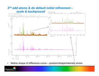
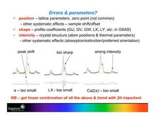
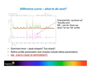
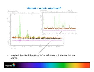
Download as PDF, PPTX
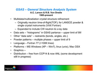
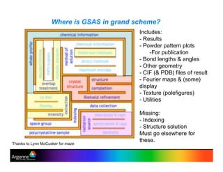
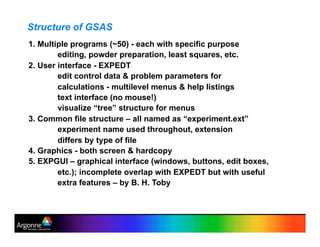
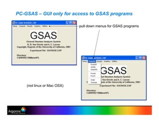
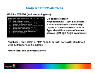
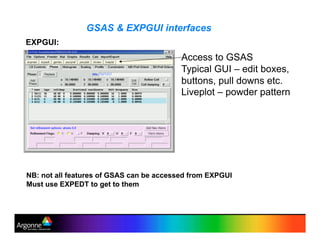
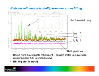
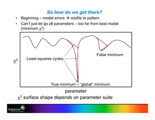
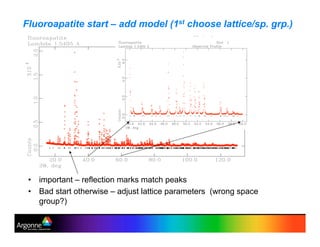

Rietveld refinement is a technique for determining crystal structures from powder diffraction data. It involves minimizing the difference between observed and calculated powder diffraction patterns through least squares refinement of structural and instrumental parameters. GSAS is a software package that performs Rietveld refinement across multiple diffraction data types. It allows refinement of parameters related to lattice constants, atomic positions, thermal motion, and instrumental profile shapes. EXPGUI provides a graphical user interface for GSAS, while EXPEDT is the text-based interface that allows access to all GSAS capabilities.