Download as PDF, PPTX
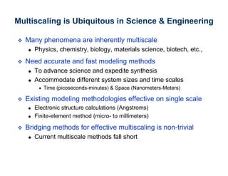
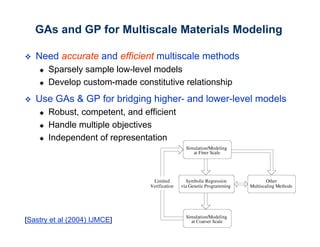
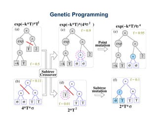
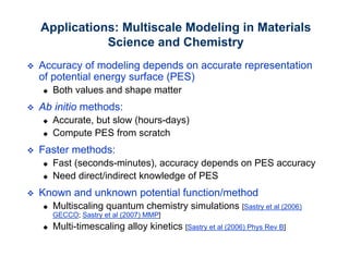
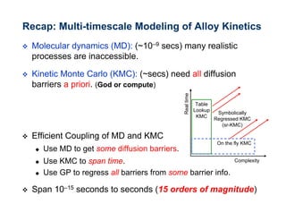
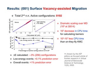
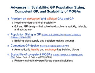

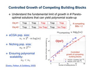
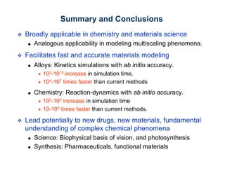
The document discusses the application of genetic algorithms (GAs) and genetic programming (GP) in multiscale modeling for materials science and chemistry, highlighting their efficiency in simulating complex phenomena across various time and space scales. Key advancements include improved scalability and the ability to bridge low- and high-level models, allowing for accurate simulations of alloy kinetics and chemical reactions. The findings indicate significant speed enhancements over traditional methods, facilitating breakthroughs in drug development and material synthesis.