1. Non-multiGaussian Multivariate Simulations
With Guaranteed Reproduction of
Inter-variable Correlations
Alastair Cornah and John Vann
Abstract Stochastic modelling of interdependent continuous spatial attributes is
now routinely carried out in the minerals industry through multiGaussian condi-
tional simulation algorithms. However, transformed conditioning data frequently
violate multiGaussian assumptions in practice, resulting in poor reproduction of cor-
relation between variables in the resultant simulations. Furthermore, the maximum
entropy property that is imposed on the multiGaussian simulations is not universally
appropriate. A new Direct Sequential Cosimulation algorithm is proposed here. In
the proposed approach, pair-wise simulated point values are drawn directly from
the discrete multivariate conditional distribution under an assumption of intrinsic
correlation with local Ordinary Kriging weights used to inform the draw proba-
bility. This generates multivariate simulations with two potential advantages over
multiGaussian methods: (1) inter-variable correlations are assured because the pair-
wise inter-variable dependencies within the untransformed conditioning data are
embedded directly into each realisation; and (2) the resultant stochastic models are
not constrained by the maximum entropy properties of multiGaussian geostatistical
simulation tools.
Alastair Cornah
Quantitative Group, PO Box 1304, Fremantle, WA, Australia 6959, e-mail: ac@qgroup.net.au.
John Vann
Quantitative Group, PO Box 1304, Fremantle, WA, Australia 6959.
Centre for Exploration Targeting, The University of Western Australia, Crawley, WA, Australia
6009.
School of Civil Environmental and Mining Engineering, The University of Adelaide, Adelaide,
SA, Australia 5000.
Cooperative Research Centre for Optimal Ore Extraction (CRC ORE), The University of Queens-
land, St. Lucia, Qld, Australia, 4067.
1

2. 2 Alastair Cornah and John Vann
1 Introduction
The advantages of stochastic modeling of in-situ mineral grade attribute variabil-
ity and geometric geological variability through conditional simulation are increas-
ingly recognised within the mining industry. Typical applications include studies
for recoverable resource estimation, mining selectivity, drill hole spacing, multi-
variate product specification, quantification of project risk through the value chain
and many others. Recent applications for conditional simulations involve feeding
multiple realizations of key attributes (grade or geometallurgical) through a virtual
mining and processing sequence in order to analyse a range of different project sce-
narios under real variability conditions. The development of such approaches means
that the demand for realistic multivariate simulations is increasing.
MultiGaussian conditional simulation algorithms, mainly the Turning Bands
Method (TBM; see Journel, 1974) and Sequential Gaussian Simulation (SGS;
Deutsch and Journel, 1992) are now widely used to simulate continuous attributes
in the minerals industry. Both these algorithms require that conditioning data hon-
our the properties of the multiGaussian model (Goovaerts, 1997) and consequently a
prior, single point, univariate transformation of the data to their normal scores equiv-
alents is therefore generally required. This ensures Gaussianity of the transformed
point attribute data, but higher order properties of the multiGaussian distribution
must also be met (Deutsch and Journel, 1998; Rivoirard, 1994; Goovaerts, 1997).
This is usually assumed to be the case, but in practice that assumption is often vio-
lated.
For most mining projects, multiple continuous interdependent attributes are of
essential interest. Examples include bulk commodity mining (iron, manganese,
coal, bauxite, phosphate, etc.); multi-element metalliferous deposits (base metals, or
base-precious metals), etc. In many mining operations deleterious components and
geometallurgical attributes are as important to financial viability and ultimate opera-
tional performance as the revenue variable(s). Because of this, reproduction of inter-
variable dependencies in realisations is as important as the reproduction of marginal
histograms for each individual variable. The traditional multivariate extension of
the multiGaussian simulation approach uses the Linear Model of Coregionalisation
(LMC) to enforce inter-variable correlations between simulated attributes (Dowd,
1971). The n inter-related random variables z1...n are transformed into their normal
scores equivalents y1...n through monotonic, univariate, single point normal scores
transforms. Multivariate pair-wise dependencies in the untransformed sample data
are also transferred into their normal scores equivalents, potentially violating the
multiGaussian assumption. Because the inverse of the normal scores transform φ −1
is also monotonic, applying the back transforms (pertaining to non-multiGaussian
sample normal score equivalents) to vector of n simulated multiGaussian distribu-
tions φ −1 (ys1...sn ) will result in multivariate pairwise dependencies in the simulated
data that are not found in the untransformed sample data; often these pairings are
mineralogically impossible. In addition, the limitations of modeling direct and cross
variograms through the LMC is well documented (Wackernagel et al. 1989; Goulard
and Voltz, 1992; Oliver, 2003).

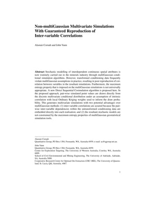
3. Non-multiGaussian Multivariate Simulations 3
Figure 1 presents the bivariate distributions between four grade variables for sam-
ple data and a back transformed multiGaussian (TBM) simulation. The black poly-
gons represent areas of bi- and multi-variate pairings in the simulated values that are
impossible due to mineralogical constraint. While the realisation generally honors
the marginal distributions of each of the variables in the conditioning data and the
general shape of the bivariate relationships, there are clearly a significant number of
mineralogically impossible pairings present in the simulation.
Fig. 1 Comparison of pairwise dependencies in the sample dataset (blue) for Al2 O3 , Fe, P and
SiO2 against simulated values (red) generated using the multiGaussian LMC approach. The black
polygons denote invalid simulated bivariate pairings.
Existing solutions to this problem within the multiGaussian framework aim to
first decorrelate the conditioning data so that it is free from multivariate non-
multiGaussian behaviors. Simulation by TBM or SGS can then be carried out
independently and the original inter-variable correlations are reconstructed post-
simulation. The Stepwise Conditional Transform (SCT) was first used in geostatis-
tics by Leuangthong and Deutsch (2003) and involves the transformation of multiple
variables to be univariate and multivariate Gaussian, with no cross correlations, un-

4. 4 Alastair Cornah and John Vann
der an assumption of intrinsic correlation. However, the method requires relatively
large datasets to be effective, can be sensitive to ordering and loses efficacy for
subsequent variables. Min-Max Autocorrelation Factors (MAF; Switzer and Green,
1984; Desbarats and Dimitrakopoulos 2000; Boucher and Dimitrakopoulos, 2009)
is a principal components based decomposition which is extended to incorporate
the spatial nature of data. However, non-linear dependencies between attributes are
problematic (Boucher and Dimitrakopoulos, 2004) and will also result in unlikely
or impossible attribute value pairings.
Nevertheless, even overlooking this issue, a well known feature of the multi-
Gaussian approach is the imposition of maximum entropy upon stochastic realiza-
tions (see Journel and Alabert, 1989). This may be pragmatically compatible with
the real deposit grade architecture for some mineralisation styles, depending on the
scale considered, but in many cases it is at least questionable. For example in Banded
Iron Formation (BIF) hosted iron ore deposits, such as those in the Pilbara region
of Australia and elsewhere, from which the example dataset is drawn, the lower
extreme of the Fe grade distribution and upper extremes of the SiO2 and Al2 O3
distributions generally comprise shale bands. These shale bands are thin relative to
standard mining selectivity and are cannot be practically separated from the rest of
the material during mining, but are far from spatially disordered. In fact individual
shale bands are continuously traceable over hundreds of kilometres and are used by
exploration and mining geologists as marker horizons to aid geological interpreta-
tions. Consequently, imposition of maximum disorder in the simulated extreme low
Fe and extreme high SiO2 and Al2 O3 values in these deposits will not only result in
poor spatial representations, it is also utterly inconsistent with important features of
the real grade architecture and known geological continuities.
Sequential Indicator Simulation (SIS; Alabert, 1987; Emery, 2004; Goovaerts,
1997) provides a potentially lower entropy alternative to the multiGaussian ap-
proach for the simulation of a single continuous attribute but no practical multivari-
ate extension is available. The requirement for a conditional simulation algorithm
which avoids the maximum entropy property and also ensures proper reproduction
of inter-variable dependencies is therefore clear. It is also clear that these two prop-
erties (maximum entropy and poor inter-variable dependency reproduction) are cou-
pled. In summary, whilst the multiGaussian assumption provides congenial proper-
ties for the simulation of an individual variable, it imposes maximum entropy on the
resulting realisations and causes difficulty in replicating non-multiGaussian inter-
variable dependencies.
2 Direct Sequential Simulation
Direct Sequential Simulation (DSS: Journel, 1994; Caers, 2000; Soares, 2001; Horta
and Soares, 2010) has been proposed to avoid the requirement for a multiGaussian
assumption and also therefore offers the possibility of lower entropy stochastic im-
ages. DSS is based upon a concept that was introduced by Journel (1994) who sub-

5. Non-multiGaussian Multivariate Simulations 5
mitted that sequential simulation will honour the covariance model whatever choice
of local conditional distribution (cdf) that simulated values are drawn from, pro-
vided that distribution is informed by the Simple Kriging (SK) mean z(xu )∗ and SK
2
variance σsk (xu ), where:
z(xu )∗ = m + ∑ λα (xu ) [z (xα ) − m]
α
and xα are the conditioning data (including sample data and previously simulated
nodes). One critical drawback was that, unless the cdf is fully defined by its mean
and variance (which is true only in the case of a few parametric distributions such
as the Gaussian), the realisation does not reproduce the input (target) histogram.
Recognising this, further development of DSS was carried out by Soares (2001)
who, instead of using z(xu )∗ and σsk (xu ) to define a local cdf from which to draw
2
zs (given a parametric assumption), zs (x ), drew directly from the (untransformed)
u
global cdf Fz (z). The draw uses a Gaussian transform φ of the original z (x) values.
The SK estimate z(xu )∗ is converted into its Gaussian equivalent y(xu )∗ and with the
standardised estimation variance this defines the sampling interval in the Gaussian
global conditional distribution:
G(y(xu )∗ , σsk (xu ))
2
The drawn Gaussian value ys is then back transformed to a simulated value zs (xu )
using the inverse of the transform φ −1 :
zs (xu ) = φ −1 (ys )
This development allowed DSS realisations to honour the target histogram as
well as the variogram. The method was extended to incorporate a secondary vari-
able, using Collocated Cokriging (Xu et al., 1992) to define the sampling of the
global conditional distribution of the secondary variable (Soares, 2001). Horta and
Soares (2010) subsequently proposed an improvement whereby the second variable
is drawn conditionally on the ranked Gaussian equivalents for the first variable. This
apparently results in improved reproduction of dependency between variables; how-
ever, the method could be progressively more problematic as the number of variables
involved increases. Furthermore, we suggest that this method still does not capital-
ize on a critical potential benefit of the direct simulation approach, which is to allow
pair-wise dependencies in the drillhole data to flow through the simulation.
3 Direct Sequential Cosimulation (DSC)
By avoiding the constraints of trying to meet multiGaussian assumptions, the di-
rect approach opens the possibility of circumventing the need to destroy and then
subsequently attempt to reconstruct inter-variable dependencies. The proposed Di-
rect Sequential Co-simulation (DSC) algorithm, which is built upon DSS, extracts

6. 6 Alastair Cornah and John Vann
pair-wise dependencies from the experimental data and embeds them directly into
the realization, thus, by construction, guaranteeing the reproduction of inter-variable
dependencies.
The DSC algorithm follows the traditional methodology for sequential simula-
tion: visiting a random sequence of nodes, estimating the local (multivariate) cu-
mulative distribution function, drawing (multivariate) values and repeating until all
nodes have been visited. As with other sequential simulation algorithms, the krig-
ing weights that are used to determine the local (multivariate) cdf must incorporate
sample data locations and previously simulated points. The drawn values are se-
quentially incorporated into the simulation until all nodes have been simulated.
In keeping with the existing DSS algorithms outlined by Horta and Soares (2010)
and summarised above, simulated data values are drawn directly from the (untrans-
formed) global conditional distribution. However, two key differences exist: (1) the
simulated data values are drawn without an intermediate Gaussian step and (2) pair-
wise multivariate simulated values for all attributes of interest are drawn directly
and simultaneously from the experimental multivariate distribution. Correlations be-
tween variables inherent within the experimental data thus become embedded within
the realizations because of the pair-wise draw and inter-variable dependencies in the
resultant simulations are assured.
The proposed DSC approach firstly requires that all variables in the sample
dataset are collocated. Secondly, an assumption of intrinsic correlation between the
attributes of interest is required. Under this assumption, direct and cross covariance
functions of all variables are proportional to the same basic spatial correlation func-
tion. In practice this is a reasonable assumption for key variables in many iron and
base metal deposits. These two requirements permit the following: at each location
to be simulated, a single set of OK weights (based upon the intrinsic spatial covari-
ance function and the geometry of data locations as well as previously simulated
nodes) can be used to define a probability mass weighting for each multivariate
pair-wise data location in the surrounding neighbourhood (simulated and sample
data) to be drawn into the simulation. This can then be utilized for the draw of pair-
wise simulated values from the experimental multivariate distribution. OK weights
are effectively used to represent the conditional probability for a pairwise value to
be drawn from the experimental multivariate distribution. This is consistent with
the interpretation of OK as an E-type (conditional expectation) estimate (Rao and
Jornel 1997) and consistent with the same author’s usage of OK weights to model
local conditional distributions.
Because OK (with unknown mean) is used instead of SK the algorithm simulates
the discrete multivariate distribution and cannot generate a value different from the
original data. In other words, in their point form, the output point simulations are
not continuous.
The DSC algorithm progresses as follows.
1. Define a random path through all nodes to be simulated.
2. For each node:

7. Non-multiGaussian Multivariate Simulations 7
OK
a. Determine local OK weights λα (u) for the surrounding experimental data
locations z(x i ) and previously simulated locations zs (xi ).
b. Sort the OK weights for each experimental and simulated data location
OK
λα (u) by magnitude and calculate the cumulative frequency weighting value
OK
C(0, 1) for each λα (u).
c. Draw a p value from a uniform distribution U(0, 1) and match to the cumu-
lative frequency C(0, 1); assign zs1...n (xu ) and add the multivariate pair-wise
values at the drawn experimental data or simulated data location to the condi-
tioning dataset.
3. Proceed to the next node along the random path and repeat steps 2a-2d until every
node has been simulated. As with other sequential simulation algorithms another
realisation is generated by repeating the entire procedure with a different random
path.
Note that OK is required in DSC because applying a probability weighting to
the mean as required by SK is impossible in the pair-wise draw sense; consequently
OK
negative weights λα (u) < 0 are a potential outcome. Because p is drawn from a
bounded uniform distribution any pair-wise data location within the neighbourhood
which is assigned a negative weight is excluded from being drawn at the simulated
location and the remaining weighting is rescaled to equal 1. The implication of this
is that in the presence of negative weights, unbiasedness in the expectation of the
simulation is not explicitly guaranteed; i.e.
E {zs (xu )} = E z (xu )∗
Other approaches, such as adding a constant positive value to all OK weights if
there is one or more negative weight, followed by restandardisation to 1 (Rao and
Journel, 1997) would also fail to guarantee unbiasedness. Our testing has shown the
impact of this to be minimal provided that estimation neighbourhood parameters
are chosen to minimise negative weights. Assuming this is the case; at each grid
location simulated values for each variable of interest are centred upon the local OK
estimate z∗ (xu ):
OK
n(u) n(u)
z∗ (xu ) =
OK
OK
∑ λα (u)z(uα ) with OK
∑ λα (u) = 1;
α=1 α=1
The range of simulated values is provided by the range of experimental and sim-
ulated data values within the search neighbourhood and the variance is the weighted
variance of the data values within the neighbourhood:
n
2
σOK (xi ) = ∑ λOK · z(xi ) − z(xu )∗
α=1
In the extreme case of no spatial continuity within the underlying geological
process, and a neighbourhood covering all of the sample data, simulated data pairs at

8. 8 Alastair Cornah and John Vann
non data locations will be drawn at random from the multivariate global conditional
distribution.
4 Example For an Iron Deposit
A two dimensional iron ore dataset which is sourced from a single geological unit
and comprises 290 exploration sample locations within a 1.2km by 1.5km mining
area is used to demonstrate the algorithm. Four grade attributes (Fe, SiO2 , Al2 O3
and P) are fully sampled across the area at an approximate spacing of 75m x 75m.
For demonstration purposes, 25 point realisations of the four attributes (Fe, SiO2 ,
Al2 O3 and P) at 19026 nodes have been generated using the proposed DSC algo-
rithm. Experimental direct variograms and cross variograms were generated for the
four variables; the direct experimental variogram for Fe was modelled using a 20%
nugget contribution and single spherical structure with 80% contribution and 200m
range. This model represents a reasonable fit to the direct SiO2 , Al2 O3 and P exper-
imental variograms when the total sill is appropriately rescaled, thereby satisfying
the intrinsic correlation requirement for the proposed DSC algorithm.
Fig. 2 A comparison between multiGaussian and DSC realisations of Fe.
A comparison between a DSC realization and a multiGaussian realization is
shown in figure 2. The grade architecture generated by DSC is more like the mosaic
model (Rivoirard, 1994; Emery, 2004) and is thus appealing in cases like the one
presented here, where maximum entropy is clearly unacceptable. A DSC realisation
of the four attributes is shown in figure 3 with the bivariate distributions between

9. Non-multiGaussian Multivariate Simulations 9
the four simulated attributes also shown. The two key advantages of the DSC algo-
rithm are apparent from the figure, specifically (1) the inter-variable relationships
in the simulated attributes match those observed in the sample dataset; and (2) the
architecture of the grades in the realization is driven by the sample data itself and
does not have the appearance of maximum entropy. In addition, by construction the
realisations honor the declustered sample histograms of the variables of interest.
Experimental direct and cross variograms for the 25 DSC realisations of the four
grade attributes are compared against their sample data equivalents in figure 4. A
close comparison is noted for both the direct and cross experimental variograms.
Ergodicity of the simulations around the sample data experimental variograms is
approximately consistent with that which might be expected from multiGaussian
algorithms.
Fig. 3 A DSC realisation of Al2 O3 , Fe, P and SiO2 with inter-simulated attribute dependencies.

10. 10 Alastair Cornah and John Vann
Distance (m)
Distance (m) Distance (m)
Distance (m) Distance (m) Distance (m)
Distance (m) Distance (m) Distance (m) Distance (m)
Fig. 4 Comparison of experimental direct and cross variograms for 25 DSC realisations of Al2 O3 ,
Fe, P and SiO2 and the sample dataset.
5 Limitations
Because the proposed DSC method simulates the discrete multivariate distribution,
simulated values cannot deviate from those in the experimental dataset. This is both
a strength of the algorithm, because it allows the pair-wise dependencies in the sam-
ple data to be embedded directly into the realizations; but it is also a weakness
because potential for simulation of adjacent nodes with the exact same value ex-
ists. This is particularly likely to be the case if the modeled spatial continuity is
high. Consequently re-blocking to change support is a critical pre-requisite to any
per realization use of the simulations with the assumption being that the averaging
process will reproduce a realistic continuous distribution at the support re-blocked
to. Prior kernel smoothing of the input data would result in a reference distribution

11. Non-multiGaussian Multivariate Simulations 11
from which to draw continuous multivariate simulated values, however this could
introduce invalid data pairings which are avoided in the algorithms’s proposed im-
plementation. A further disadvantage of the DSC approach over the multiGaussian
approach is that unlike the latter (see Deraisme et al., 2008), no direct block equiv-
alent is available. This is not a drawback from small simulations, but is a potential
restriction for large scale mining problems.
6 Conclusions
Applications of conditional simulation within the minerals industry rely directly
upon the integrity of the simulated architecture of those in situ attributes. Ade-
quately representing the connectivity of extremes of attribute distributions is critical
because very often these are the key drivers of value or causes of interaction with
mining, processing, or product specification constraints; adequate representation of
inter-attribute dependencies is equally important. The authors believe that these re-
quirements demand the ongoing development of conditional simulation algorithms
for continuous multivariate attributes outside the of the multiGaussian framework.
The DSC algorithm presented is intended to contribute to this effort by providing a
low entropy alternative to the multiGaussian approach for the conditional simulation
of multiple continuous attributes that also guarantees that inter-variable dependen-
cies are honored.
The intrinsic correlation, full sampling and collocation of sampling requirements
of DSC are no more onerous than those of SCT and in general the practical imple-
mentation of DSC is far more straightforward than the multivariate multiGaussian
approaches. No LMC modeling is required and the additional transformations and
associated validation steps that are required in MAF and the SCT are also avoided.
Acknowledgements Professor Julian Ortiz of the University of Chile and our Quantitative Group
colleagues, in particular Mike Stewart, are thanked for feedback and discussions about the pro-
posed method prior to the writing of this paper. Any remaining deficiencies are entirely the respon-
sibility of the authors.
References
1. Alabert F, 1987. Stochastic imaging of spatial distributions using hard and soft information:
Unpublished master’s thesis, Department of Applied Earth Sciences, Stanford University,
Stanford, California.
2. Boucher A and Dimitrakopoulos R, 2004. A new joint simulation framework and application
in a multivariate deposit. In Dimitrakopoulos R and Ramazan S (eds), Orebody Modelling and
Strategic Mine Planning, Perth, WA, 2004.
3. Boucher A and Dimitrakopoulos R, 2009. Block simulation of multiple correlated variables.
Mathematical Geoscience, 41(2):215-237.

12. 12 Alastair Cornah and John Vann
4. Caers J, 2000. Direct sequential indicator simulation: Proceedings of 6th International Geo-
statistics Congress, Cape Town, South Africa.
5. Deraisme J, Rivoirard J and Carrasco Castelli P, 2008. Multivariate uniform conditioning and
block simulations with discrete Gaussian model: application to Chuquicamata deposit. In Ortiz
J and Emery X (eds), Proceedings of the Eight International Geostatistics Congress pp. 69-78.
6. Desbarats A and Dimitrakopoulos, R, 2000. Geostatistical simulation of regionalized pore-size
distributions using min/max autocorrelation factors. Mathematical Geology 32(8):919-942.
7. Deutsch C, and Journel A, 1992. GSLIB–Geostatistical Software Library and user’s guide:
Oxford University Press, New York.
8. Deutsch C and Journel A, 1998. GSLIB: Geostatistical Software Library and User’s Gude:
2nd edition. Oxford University Press, New York.
9. Dowd P, 1971. The Application of geostatistics to No. 20 Level, New Broken Hill Consoli-
dated Ltd. Operations Research Department, Zinc Corporation, Conzinc Riotinto of Australia
(CRA), Broken Hill, NSW, Australia.
10. Emery X, 2004. Properties and limitations of sequential indicator simulation. Stochastic En-
vironmental Research and Risk Assessment 18:414-424.
11. Goulard M and Voltz M, 1992, Linear coregionalization model: tools for estimation and choice
of cross – variogram matrix. Mathematical Geology 24(3):269-285.
12. Goovaerts P, 1997. Geostatistics for Natural Resources Evaluation: Oxford University Press,
New York.
13. Horta A and Soares A, 2010. Direct sequential co-simulation with joint probability distribu-
tion. Mathematical Geosciences 42(3):269-292
14. Journel A, 1974. Geostatistics for conditional simulation of ore bodies. Economic Geology
69(5):673-687.
15. Journel A and Alabert F, 1989. Non-Gaussian data expansion in the earth sciences. Terra Nova
Volume 1 pp. 123-134 16.
16. Journel A, 1994. Modeling uncertainty: some conceptual thoughts, in Dimitrakopoulos R.
(ed.), Geostatistics for the Next Century: Kluwer Academic Pulications, Dordrecht, The
Netherlads 30-43.
17. Leuangthong O and Deutsch C, 2003. Stepwise conditional transformation for simulation of
multiple variables. Mathematical Geology 35(2):155-173.
18. Oliver D, 2003, Gaussian cosimulation: modeling of the cross-covariance. Mathematical Ge-
ology 35(6):681-698.
19. Rao S and Journel A, 1997. Deriving conditional distributions from ordinary kriging. In Baafi
E and Schofield N (eds.), Geostatistics – Wollongong 96: Kluwer Academic Publishers, Lon-
don 92-102
20. Rivoirard J, 1994. Introduction to Disjunctive Kriging and Non-Linear Geostatistics. Claren-
don Press (Oxford).
21. Soares A, 2001. Direct sequential simulation and co-simulation. Mathematical Geology.
33(8):911-926
22. Switzer P and Green A, 1984. Min/max autocorellation factors for multivariate spatial im-
agery. Stanford University, Department of Statistics.
23. Wackernagel H, Petigas P, and Touffait Y, 1989, Overview of methods for coregionalisation
analysis. I Armstrong M (ed.) Geostatistics Vol. 1: 409-420 23. Xu W, Tran T, Srivastava RM
and Journel A, 1992. Integrating seismic data in reservoir modeling: The collocated cokriging
alternative. SPE 24742