SlideShare a Scribd company logo
1 of 6
Download to read offline
Simultaneous TV-regularized time-lapse FWI with application to field data
Musa Maharramov∗, Biondo Biondi, Stanford University, and Mark Meadows, Chevron Energy Technology Company
SUMMARY
We present a field data application of the technique pro-
posed by Maharramov and Biondi (2015) for reconstruct-
ing production-induced subsurface model changes from time-
lapse seismic data using full-waveform inversion (FWI). The
technique simultaneously inverts multiple survey vintages with
total-variation (TV) regularization of the model differences.
After describing the method, we discuss its application to the
Gulf of Mexico, Genesis Field data. We resolve negative ve-
locity changes associated with overburden dilation and demon-
strate that the results are stable with respect to the amount
of regularization and consistent with earlier estimates of time
strain in the overburden.
INTRODUCTION
Prevalent practice of time-lapse seismic processing relies on
picking time displacements and changes in reflectivity ampli-
tudes between migrated baseline and monitor images, and con-
verting them into impedance changes and subsurface defor-
mation (Johnston, 2013). This approach requires a significant
amount of manual interpretation and quality control. An al-
ternative approach is based on using the high-resolution power
of full-waveform inversion (Sirgue et al., 2010a) to reconstruct
production-induced changes from wide-offset seismic acquisi-
tions (Routh et al., 2012; Zheng et al., 2011; Asnaashari et al.,
2012; Raknes et al., 2013; Maharramov and Biondi, 2014a;
Yang et al., 2014). However, while potentially reducing the
amount of manual interpretation, time-lapse FWI is sensitive
to repeatability issues (Asnaashari et al., 2012), with both co-
herent and incoherent noise potentially masking important pro-
duction-induced changes. The joint time-lapse FWI proposed
by Maharramov and Biondi (2013, 2014a) addressed repeata-
bility issues by joint inversion of multiple vintages with model-
difference regularization based on the L2-norm and produced
improved results when compared to the conventional time-lapse
FWI techniques. Maharramov and Biondi (2015) extended
this joint inversion approach to include edge-preserving total-
variation (TV) model-difference regularization. The new me-
thod was shown to achieve a dramatic improvement over alter-
native techniques by significantly reducing oscillatory artifacts
in the recovered model difference for synthetic data with re-
peatability issues. In this work, we apply this TV-regularized
simultaneous inversion technique to the Gulf of Mexico, Gene-
sis Field data and demonstrate a stable recovery of production-
induced model changes.
METHOD
FWI applications in time-lapse problems seek to recover in-
duced changes in the subsurface model by using multiple seis-
mic datasets from different acquisition vintages. For two sur-
veys sufficiently separated in time, we call such datasets (and
the associated models) “baseline” and “monitor”. Time-lapse
FWI can be conducted by separately inverting the baseline and
monitor models (“parallel difference”, Plessix et al. (2010)) or
inverting them sequentially with, e.g., the baseline supplied as
a starting model for the monitor inversion (“sequential differ-
ence”). The latter may achieve a better recovery of model dif-
ferences in the presence of incoherent noise (Asnaashari et al.,
2012; Maharramov and Biondi, 2014a). Another alternative
is to apply the “double-difference” method (Watanabe et al.,
2004; Denli and Huang, 2009; Zheng et al., 2011; Asnaashari
et al., 2012; Raknes et al., 2013). The latter approach may
require significant data pre-processing and equalization (As-
naashari et al., 2012; Maharramov and Biondi, 2014a) across
survey vintages.
Figure 1: A north-south inline section of the baseline image
produced by Chevron (vertical axis two-way travel time in sec-
onds, horizontal axis inline meters).
In all of these techniques, optimization is conducted with re-
spect to one model at a time, albeit of different vintages at dif-
ferent stages of the inversion. We propose to invert the baseline
and monitor models simultaneously by solving the following
optimization problem (Maharramov and Biondi, 2015):
α ub(mb)−db
2
2 +β um(mm)−dm
2
2 + (1)
δ WR(mm −mb) 1 → min (2)
with respect to both the baseline and monitor models mb and
mm. Problem (1,2) describes time-lapse FWI with the L1 reg-
ularization of the transformed model difference (2). The terms
(1) correspond to separate baseline and monitor inversions with
observed data d and modeled data u. In (2), R and W denote
regularization and weighting operators, respectively. If R is
the gradient magnitude operator
Rf(x,y,z) = f2
x + f2
y + f2
z , (3)
then (2) becomes the “Total Variation” (TV) seminorm. The
latter case is of particular interest, because minimization of
the gradient L1 norm promotes “blockiness” of the model-
difference, potentially reducing oscillatory artifacts (Rudin et al.,
1992). Total-variation regularization, known in image process-
ing as the “ROF Model”, was applied earlier to full-waveform
SEG New Orleans Annual Meeting Page 1236
DOI http://dx.doi.org/10.1190/segam2015-5925444.1© 2015 SEG
Downloaded08/22/15to128.12.158.51.RedistributionsubjecttoSEGlicenseorcopyright;seeTermsofUseathttp://library.seg.org/
Application of joint TV-regularized 4D FWI
inversion as a way of resolving sharp geologic boundaries (Ana-
gaw and Sacchi, 2012). The solution of a large-scale opti-
mization problem based on the ROF model using conventional
methods is computationally challenging, prone to the “stair-
casing effect” (Chambolle and Lions, 1997), and may require
solution methods that involve splitting and gradient threshold-
ing (Goldstein and Osher, 2009). However, time-lapse FWI
appears to be a nearly ideal application for the ROF model, be-
cause significant production-induced subsurface model changes
are spatially bounded and have magnitudes that can be roughly
estimated a priori from geomechanical and production data
(Maharramov and Biondi (2014a), supplementary material).
More specifically, the weighting operator W may be obtained
from prior geomechanical information. For example, a rough
estimate of production-induced velocity changes can be ob-
tained from time shifts (Hatchell and Bourne, 2005) and used
to map subsurface regions of expected production-induced per-
turbation.
Figure 2: Monitor and baseline image-difference obtained
from the 3D time-migration images provided by Chevron and
corresponding to the inline section of Figure 1. Production-
induced changes stand out at approximately 3.5 s (wet Illi-
noisan sands) and 4 s two-way travel times—stacked Neb 1,
2, and 3 reservoirs—compare with Hudson et al. (2005).
APPLICATION TO FIELD DATA
The Genesis Field, operated by Chevron, is located 150 miles
southwest of New Orleans in the Green Canyon area of the
central Gulf of Mexico, in approximately 770-830m of water
(Magesan et al., 2005). Oil was found in several late Pliocene
through early Pleistocene deep-water reservoirs. Most of the
field’s oil and gas reserves are in the early Pleistocene Neb 1,
Neb 2, and Neb 3 reservoirs that are the primary subject of this
study. First oil production began in January 1999.
A 3D seismic survey was shot in 1990, and a time-lapse survey
was shot in October 2002 with the aim of improving field man-
agement (Hudson et al., 2005; Magesan et al., 2005). Cumu-
lative production from the field at the time of the monitor sur-
vey was more than 57 MMBO, 89 MMCFG, and 19 MMBW
(Hudson et al., 2005).
In addition to fluid substitution effects, producing reservoirs
compact, increasing the depth to the top of the reservoirs and
causing overburden dilation (Johnston, 2013). A time-lapse
study performed by Chevron (Hudson et al., 2005) indicated
significant apparent kinematic differences in the Pleistocene
reservoir interval. Time shifts were observed both for the pro-
ducing reservoirs and Illinoisan wet sands above Neb 1 (see
Figure 3). Kinematic differences were attributed to a time shift
caused by subsidence at the top of the uppermost reservoir,
subsidence of the overburden, and overburden dilation (Hud-
son et al., 2005).
Figure 3: Production-induced changes resulted in measurable
time-shifts between the surveys. Shown here are time-shifts
between the baseline (blue) and monitor (red) common-offset
gathers, 1074 m offset.
Parameters of the baseline and monitor surveys and subsequent
time-lapse processing by Chevron were described by Magesan
et al. (2005). The baseline survey had a maximum offset of
5 km, and the monitor survey had a maximum offset of 7.3
km. Both surveys had a bin size of 12.5 m by 37 m. For the
purpose of time-lapse analysis, the acquired data had been sub-
jected to data equalization, pre-processing and imaging steps
that included a spherical divergence correction, source and re-
ceiver statics, global phase rotation, time shift, amplitude scal-
ing, global spectral matching, and cross-equalization (Mage-
san et al., 2005).
The data pre-processed for time-lapse analysis were used by
Chevron in Kirchhoff time migration of the baseline and mon-
itor surveys, producing 3D images. A single inline section of
the baseline image is shown in Figure 1. The corresponding
monitor and baseline image difference is shown in Figure 2.
As noted by Hudson et al. (2005), the image difference is con-
tributed to by time shifts at the Illinoisan sands (upper event)
and Neb 1 (lower event) in Figure 2—compare with Figure 1
of Hudson et al. (2005).
The purpose of this exercise was to verify whether or not joint
regularized time-lapse FWI could resolve some of the pro-
duction-induced model differences, thus providing additional
insight into reservoir depletion patterns and optimal infill dril-
ling strategies. As our first processing step, we performed sep-
arate baseline and monitor 2D full-waveform inversion of a
single inline section. We extracted a single north-south inline
corresponding to the image in Figure 1 from both surveys and
SEG New Orleans Annual Meeting Page 1237
DOI http://dx.doi.org/10.1190/segam2015-5925444.1© 2015 SEG
Downloaded08/22/15to128.12.158.51.RedistributionsubjecttoSEGlicenseorcopyright;seeTermsofUseathttp://library.seg.org/
Application of joint TV-regularized 4D FWI
Figure 4: Inverted baseline velocity model. FWI resolved fine
model features and oriented them along the dip structure of the
image in Figure 1 (vertical axis depth meters).
sorted it into shot gathers with a minimum offset of 350 m and
a maximum offset of 4,700 m, 1,264 shots and up to 175 re-
ceivers per shot. A frequency-domain 2D FWI (Sirgue et al.,
2008, 2010b) was conducted over the frequency range of 3-
30.7 Hz. Frequency spacing was selected using the technique
of Sirgue and Pratt (2004). The data provided to us had under-
gone amplitude pre-processing that included a spherical diver-
gence correction. Furthermore, accurate handling of the am-
plitudes in 2D FWI of 3D field data requires a 3D-to-2D data
transformation (Auer et al., 2013). Because the data exhib-
ited significant time-shifts at the reservoir level (Hudson et al.,
2005) that can be readily observed even at far offsets (see Fig-
ure 3), we decided to use a “phase-only” inversion and ignored
amplitude information in the data (Fichtner, 2011).
The result of baseline inversion is shown in Figure 4. To build
a starting model for the FWI, we converted Chevron’s RMS
time-migration velocity model to an interval velocity using the
Dix equation, and smoothed the result using a triangular filter
with a 41-sample window. Observe that FWI succeeded in re-
solving fine features, and oriented them consistently along the
dip structure of the time-migrated image in Figure 1. Close-up
views of the model area covering both the Illinoisan sands and
the reservoirs are shown in Figures 6a and 6c.
The result of parallel differencing is shown in Figure 5a. Al-
though significant model changes appear to be concentrated
around the target area, this result is not interpretable, either
qualitatively or quantitatively, because it is contaminated with
oscillatory artifacts and overestimates the magnitudes of ve-
locity perturbations. This result is consistent with our earlier
assessment of conventional time-lapse FWI techniques tested
on synthetic data (Maharramov and Biondi, 2014a, 2015).
Next, we solved the simultaneous, TV-regularized time-lapse
full-waveform inversion problem (1,2). We set α = β = 1 and
carried out multiple experiments with the value of the regular-
ization parameter δ ranging from δ = 100 to δ = 1000. The
weighting operator W was set to 1 inside the larger target area
shown in Figures 5a through 6b, tapering off to zero outside.
The results of inverting the model difference for δ = 100, 500
and 1000 are shown in Figures 5b, 5c, and 5d, respectively.
Gradual increase of the regularization parameter results in the
removal of most model differences with the exception of a neg-
ative velocity perturbation in the overburden, peaking at ap-
proximately 3.6 km and 3.9 km (see Figures 6b and 6d). Such
perturbations are consistent with overburden dilation due to
the compaction of stacked reservoirs, with more significant di-
lation in the wet Illinoisan sands than the surrounding shales
(Rickett et al., 2007). The zone of negative velocity change
appears to extend upward into the overburden in a direction
roughly orthogonal to the reservoir dip—see Figure 5d. Two
negative velocity changes at approximately 10 and 11.5 km in-
line persist with increasing regularization, and may represent
dilation effects associated with the production from deeper re-
servoirs—compare with Figure 3 of Rickett et al. (2007).
The estimated maximum negative velocity change of −45 m/s
above the stacked reservoirs is consistent with the earlier es-
timates of time strain in the overburden (Rickett et al., 2007).
Indeed, local time strain, physical strain and partial velocity
change are related by the equation (Hatchell and Bourne, 2005)
dτ
dt
≈
∆t
t
=
∆z
z
−
∆v
v
, (4)
where τ,t,z, and v denote the observed time shift, travel time,
depth, and velocity. Assuming, following Hatchell and Bourne
(2005), that
∆v
v
= −R
∆z
z
, (5)
where the factor R is estimated to be 6 ± 2 for the Genesis
overburden (Hodgson et al., 2007), we obtain
∆v
v
= −
R
R+1
∆t
t
≈ −
∆t
t
≈ −
dτ
dt
. (6)
Maximum time strains in the Genesis overburden are estimated
to be around +2% (Rickett et al., 2007), yielding the maximum
negative velocity change of
∆v ≈ −.02×2,800 m/s = −56 m/s, (7)
where the estimated P-wave velocity of 2,800 m/s at a 3.6 km
depth was taken from the output of our FWI.
CONCLUSIONS
Simultaneous time-lapse FWI with total-variation difference
regularization can achieve robust recovery of production-in-
duced changes, preserving the blocky nature of monitor-base-
line differences. Velocity changes caused by overburden dila-
tion are within the resolution of our method. However, veloc-
ity changes within thin reservoirs (e.g., caused by compaction)
can no longer be characterized as “blocky” on a seismic scale,
and recovering such changes may require a multi-norm model
decomposition approach a la Maharramov and Biondi (2014b),
and will be the subject of further research.
ACKNOWLEDGMENTS
The authors would like to thank the affiliate members of Stan-
ford Exploration Project (SEP) for their support; Joseph Ste-
fani, Stewart Levin, Shuki Ronen, and Dimitri Bevc for a num-
ber of useful discussions; Chevron for providing the field data;
and the Stanford Center for Computational Earth and Environ-
mental Science for providing computing resources.
SEG New Orleans Annual Meeting Page 1238
DOI http://dx.doi.org/10.1190/segam2015-5925444.1© 2015 SEG
Downloaded08/22/15to128.12.158.51.RedistributionsubjecttoSEGlicenseorcopyright;seeTermsofUseathttp://library.seg.org/
Application of joint TV-regularized 4D FWI
(a) (b)
(c) (d)
Figure 5: (a) Parallel difference and joint inversion results for (b) δ = 100, (c) δ = 500, and (d) δ = 1000 in the target area. Note
that the parallel difference result is not interpretable because of the presence of artifacts. Increasing the regularization parameter
δ results in gradual removal of most model differences except the negative velocity change in the overburden, peaking around the
Illinoisan sands and near the top of the stacked reservoirs—see Figures 6a through 6d.
(a) (b)
(c) (d)
Figure 6: (a) Baseline target area and (b) estimated model difference for δ = 1000. Close-up of (c) baseline target area and (b)
estimated model difference for δ = 1000.
SEG New Orleans Annual Meeting Page 1239
DOI http://dx.doi.org/10.1190/segam2015-5925444.1© 2015 SEG
Downloaded08/22/15to128.12.158.51.RedistributionsubjecttoSEGlicenseorcopyright;seeTermsofUseathttp://library.seg.org/
EDITED REFERENCES
Note: This reference list is a copyedited version of the reference list submitted by the author. Reference lists for the 2015
SEG Technical Program Expanded Abstracts have been copyedited so that references provided with the online metadata for
each paper will achieve a high degree of linking to cited sources that appear on the Web.
REFERENCES
Anagaw, A. Y., and M. D. Sacchi, 2012, Edge-preserving seismic imaging using the total variation
method: Journal of Geophysics and Engineering, 9, no. 2, 138–
146. http://dx.doi.org/10.1088/1742-2132/9/2/138.
Asnaashari, A., R. Brossier, S. Garambois, F. Audebert, P. Thore, and J. Virieux, 2012, Time-lapse
imaging using regularized FWI: A robustness study: 82nd Annual International Meeting, SEG,
Expanded Abstracts, doi:http://dx.doi.org/10.1190/segam2012-0699.1.
Auer, L., A. M. Nuber, S. A. Greenhalgh, H. Maurer, and S. Marelli, 2013, A critical appraisal of
asymptotic 3D-to-2D data transformation in full-waveform seismic crosshole tomography:
Geophysics, 78, no. 6, R235–R247. http://dx.doi.org/10.1190/geo2012-0382.1.
Chambolle, A., and P. L. Lions, 1997, Image recovery via total variational minimization and related
problems: Numerische Mathematik, 76, no. 2, 167–
188. http://dx.doi.org/10.1007/s002110050258.
Denli, H., and L. Huang, 2009, Double-difference elastic waveform tomography in the time domain: 79th
Annual International Meeting, SEG, Expanded Abstracts, 2302–2306.
Fichtner, A., 2011, Full-seismic modeling and inversion: Springer. http://dx.doi.org/10.1007/978-3-642-
15807-0.
Goldstein, T., and S. Osher, 2009, The split Bregman method for L1-regularized problems: SIAM Journal
on Imaging Sciences, 2, no. 2, 323–343. http://dx.doi.org/10.1137/080725891.
Hatchell, P., and S. Bourne, 2005, Measuring reservoir compaction using time-lapse time shifts: 75th
Annual International Meeting, SEG, Expanded Abstracts, 2500–2503.
Hodgson, N., C. Macbeth, L. Duranti, J. Rickett, and K. Nihei, 2007, Inverting for reservoir pressure
change using time-lapse time strain: Application to Genesis Field, Gulf of Mexico: The Leading
Edge, 26, 649–652. http://dx.doi.org/10.1190/1.2737104.
Hudson, T., B. Regel, J. Bretches, J. Rickett, B. Cerney, and P. Inderwiesen, 2005, Genesis Field, Gulf of
Mexico, 4D project status and preliminary lookback: 75th Annual International Meeting, SEG,
Expanded Abstracts, 2436–2439.
Johnston, D., 2013, Practical applications of time-lapse seismic data:
SEG. http://dx.doi.org/10.1190/1.9781560803126.
Magesan, M., S. Depagne, K. Nixon, B. Regel, J. Opich, G. Rogers, and T. Hudson, 2005, Seismic
processing for time-lapse study: Genesis Field, Gulf of Mexico: The Leading Edge, 24, 364–
373. http://dx.doi.org/10.1190/1.1901384.
Maharramov, M., and B. Biondi, 2013, Simultaneous time-lapse full-waveform inversion: SEP Report,
150, 63–70.
Maharramov, M., and B. Biondi, 2014a, Joint full-waveform inversion of time-lapse seismic data sets:
84th Annual Meeting, SEG, Expanded Abstracts, 954–959.
Maharramov, M., and B. Biondi, 2014b, Multimodel full-waveform inversion: SEP Report, 155, 187–
192.
SEG New Orleans Annual Meeting Page 1240
DOI http://dx.doi.org/10.1190/segam2015-5925444.1© 2015 SEG
Downloaded08/22/15to128.12.158.51.RedistributionsubjecttoSEGlicenseorcopyright;seeTermsofUseathttp://library.seg.org/
Maharramov, M., and B. Biondi, 2015, Robust simultaneous time-lapse full-waveform inversion with
total-variation regularization of model difference: 77th Annual International Conference and
Exhibition, EAGE, Extended Abstracts, http://dx.doi.org/10.3997/2214-4609.201413085.
Plessix, R.-E., S. Michelet, H. Rynja, H. Kuehl, C. Perkins, J. W. de Maag, and P. Hatchell, 2010, Some
3D applications of full waveform inversion: Presented at the 72nd Annual International
Conference and Exhibition, EAGE, Workshop WS6 3D Full-Waveform Inversion — A Game-
Changing Technique?.
Raknes, E., W. Weibull, and B. Arntsen, 2013, Time-lapse full-waveform inversion: Synthetic and real
data examples: 83rd Annual International Meeting, SEG, Expanded Abstracts, 944–948.
Rickett, J., L. Duranti, T. Hudson, B. Regel, and N. Hodgson, 2007, 4D time strain and the seismic
signature of geomechanical compaction at Genesis: The Leading Edge, 26, 644–647.
http://dx.doi.org/10.1190/1.2737103.
Routh, P., G. Palacharla, I. Chikichev, and S. Lazaratos, 2012, Full-wavefield inversion of time-lapse data
for improved imaging and reservoir characterization: 82nd Annual International Meeting, SEG,
Expanded Abstracts, doi:http://dx.doi.org/10.1190/segam2012-1043.1., 1–6.
Rudin, L. I., S. Osher, and E. Fatemi, 1992, Nonlinear total variation based noise removal algorithms:
Physica D. Nonlinear Phenomena, 60, no. 1–4, 259–268. http://dx.doi.org/10.1016/0167-
2789(92)90242-F.
Sirgue, L., O. Barkved, J. Dellinger, J. Etgen, U. Albertin, and J. Kommendal, 2010a, Full-waveform
inversion: The next leap forward in imaging at Valhall: First Break, 28, no. 4, 65–70.
Sirgue, L., J. T. Etgen, and U. Albertin, 2008, 3D frequency domain waveform inversion using time
domain finite difference methods: 70th Annual International Conference and Exhibition, EAGE,
Extended Abstracts, http://dx.doi.org/10.3997/2214-4609.20147683.
Sirgue, L., J. T. Etgen, U. Albertin, and S. Brandsberg-Dahl, 2010b, System and method for 3D frequency
domain waveform inversion based on 3D time-domain forward modeling: U. S. Patent 7,725,266.
Sirgue, L., and R. Pratt, 2004, Efficient waveform inversion and imaging: A strategy for selecting
temporal frequencies: Geophysics, 69, 231–248. http://dx.doi.org/10.1190/1.1649391.
Watanabe, T., S. Shimizu, E. Asakawa, and T. Matsuoka, 2004, Differential waveform tomography for
time-lapse crosswell seismic data with application to gas hydrate production monitoring: 74th
Annual International Meeting, SEG, Expanded Abstracts, 2323–2326.
Yang, D., A. E. Malcolm, and M. C. Fehler, 2014, Time-lapse full-waveform inversion and uncertainty
analysis with different survey geometries: 76th Annual International Conference and Exhibition,
EAGE, Extended Abstracts, http://dx.doi.org/10.3997/2214-4609.20141120.
Zheng, Y., P. Barton, and S. Singh, 2011, Strategies for elastic full-waveform inversion of time-lapse
ocean bottom cable (OBC) seismic data: 81st Annual International Meeting, SEG, Expanded
Abstracts, 4195–4200.
SEG New Orleans Annual Meeting Page 1241
DOI http://dx.doi.org/10.1190/segam2015-5925444.1© 2015 SEG
Downloaded08/22/15to128.12.158.51.RedistributionsubjecttoSEGlicenseorcopyright;seeTermsofUseathttp://library.seg.org/

More Related Content

What's hot

3 d numerical modeling of supercritical flow in gradual expansions
3 d numerical modeling of supercritical flow in gradual expansions3 d numerical modeling of supercritical flow in gradual expansions
3 d numerical modeling of supercritical flow in gradual expansionsPercy Rosales
 
Geological mapping using satellite images.
Geological mapping using satellite images.Geological mapping using satellite images.
Geological mapping using satellite images.Diego Bedoya Gonzalez
 
Modelling of 3D gelogical structures
Modelling of 3D gelogical structuresModelling of 3D gelogical structures
Modelling of 3D gelogical structuresZawar Khan
 
Assessing 50 years of tropical Peruvian glacier volume change from multitempo...
Assessing 50 years of tropical Peruvian glacier volume change from multitempo...Assessing 50 years of tropical Peruvian glacier volume change from multitempo...
Assessing 50 years of tropical Peruvian glacier volume change from multitempo...InfoAndina CONDESAN
 
Prediction of scour depth at bridge abutments in cohesive bed using gene expr...
Prediction of scour depth at bridge abutments in cohesive bed using gene expr...Prediction of scour depth at bridge abutments in cohesive bed using gene expr...
Prediction of scour depth at bridge abutments in cohesive bed using gene expr...Mohd Danish
 
Scour prediction at bridge piers in cohesive bed using gene expression progra...
Scour prediction at bridge piers in cohesive bed using gene expression progra...Scour prediction at bridge piers in cohesive bed using gene expression progra...
Scour prediction at bridge piers in cohesive bed using gene expression progra...Mohd Danish
 
Day 1 - a.p. dimri, jawaharlal nehru university, india, arrcc-carissa workshop
Day 1 - a.p. dimri, jawaharlal nehru university, india, arrcc-carissa workshopDay 1 - a.p. dimri, jawaharlal nehru university, india, arrcc-carissa workshop
Day 1 - a.p. dimri, jawaharlal nehru university, india, arrcc-carissa workshopICIMOD
 
Prediction of scour depth at bridge abutments in cohesive bed using gene expr...
Prediction of scour depth at bridge abutments in cohesive bed using gene expr...Prediction of scour depth at bridge abutments in cohesive bed using gene expr...
Prediction of scour depth at bridge abutments in cohesive bed using gene expr...IAEME Publication
 
20160602 Non-Invasive Geophysical Techniques
20160602 Non-Invasive Geophysical Techniques20160602 Non-Invasive Geophysical Techniques
20160602 Non-Invasive Geophysical TechniquesSam Setchell
 
Heritage hetherington lidar_pdf[1]
Heritage hetherington lidar_pdf[1]Heritage hetherington lidar_pdf[1]
Heritage hetherington lidar_pdf[1]llica
 
Development of Methodology for Determining Earth Work Volume Using Combined S...
Development of Methodology for Determining Earth Work Volume Using Combined S...Development of Methodology for Determining Earth Work Volume Using Combined S...
Development of Methodology for Determining Earth Work Volume Using Combined S...IJMER
 
2010 rock slope risk assesment based on geostructural anna
2010 rock slope risk assesment based on geostructural anna2010 rock slope risk assesment based on geostructural anna
2010 rock slope risk assesment based on geostructural annaMasagus Azizi
 
2D MASW ANALYSIS FOR GEOTECHNICAL ENGINEERING
2D MASW ANALYSIS FOR GEOTECHNICAL ENGINEERING2D MASW ANALYSIS FOR GEOTECHNICAL ENGINEERING
2D MASW ANALYSIS FOR GEOTECHNICAL ENGINEERINGAli Osman Öncel
 
_GC2014_Integration_of_Geologic_Data_into_Structural_Imaging
_GC2014_Integration_of_Geologic_Data_into_Structural_Imaging_GC2014_Integration_of_Geologic_Data_into_Structural_Imaging
_GC2014_Integration_of_Geologic_Data_into_Structural_ImagingDennis Ellison
 
Velocity Models Difference
Velocity Models DifferenceVelocity Models Difference
Velocity Models DifferenceShah Naseer
 
ÖNCEL AKADEMİ: INTRODUCTION TO GEOPHYSICS
ÖNCEL AKADEMİ: INTRODUCTION TO GEOPHYSICSÖNCEL AKADEMİ: INTRODUCTION TO GEOPHYSICS
ÖNCEL AKADEMİ: INTRODUCTION TO GEOPHYSICSAli Osman Öncel
 

What's hot (18)

3 d numerical modeling of supercritical flow in gradual expansions
3 d numerical modeling of supercritical flow in gradual expansions3 d numerical modeling of supercritical flow in gradual expansions
3 d numerical modeling of supercritical flow in gradual expansions
 
Geological mapping using satellite images.
Geological mapping using satellite images.Geological mapping using satellite images.
Geological mapping using satellite images.
 
Modelling of 3D gelogical structures
Modelling of 3D gelogical structuresModelling of 3D gelogical structures
Modelling of 3D gelogical structures
 
Assessing 50 years of tropical Peruvian glacier volume change from multitempo...
Assessing 50 years of tropical Peruvian glacier volume change from multitempo...Assessing 50 years of tropical Peruvian glacier volume change from multitempo...
Assessing 50 years of tropical Peruvian glacier volume change from multitempo...
 
Prediction of scour depth at bridge abutments in cohesive bed using gene expr...
Prediction of scour depth at bridge abutments in cohesive bed using gene expr...Prediction of scour depth at bridge abutments in cohesive bed using gene expr...
Prediction of scour depth at bridge abutments in cohesive bed using gene expr...
 
Scour prediction at bridge piers in cohesive bed using gene expression progra...
Scour prediction at bridge piers in cohesive bed using gene expression progra...Scour prediction at bridge piers in cohesive bed using gene expression progra...
Scour prediction at bridge piers in cohesive bed using gene expression progra...
 
Day 1 - a.p. dimri, jawaharlal nehru university, india, arrcc-carissa workshop
Day 1 - a.p. dimri, jawaharlal nehru university, india, arrcc-carissa workshopDay 1 - a.p. dimri, jawaharlal nehru university, india, arrcc-carissa workshop
Day 1 - a.p. dimri, jawaharlal nehru university, india, arrcc-carissa workshop
 
Prediction of scour depth at bridge abutments in cohesive bed using gene expr...
Prediction of scour depth at bridge abutments in cohesive bed using gene expr...Prediction of scour depth at bridge abutments in cohesive bed using gene expr...
Prediction of scour depth at bridge abutments in cohesive bed using gene expr...
 
20160602 Non-Invasive Geophysical Techniques
20160602 Non-Invasive Geophysical Techniques20160602 Non-Invasive Geophysical Techniques
20160602 Non-Invasive Geophysical Techniques
 
Heritage hetherington lidar_pdf[1]
Heritage hetherington lidar_pdf[1]Heritage hetherington lidar_pdf[1]
Heritage hetherington lidar_pdf[1]
 
Development of Methodology for Determining Earth Work Volume Using Combined S...
Development of Methodology for Determining Earth Work Volume Using Combined S...Development of Methodology for Determining Earth Work Volume Using Combined S...
Development of Methodology for Determining Earth Work Volume Using Combined S...
 
A05740104
A05740104A05740104
A05740104
 
2010 rock slope risk assesment based on geostructural anna
2010 rock slope risk assesment based on geostructural anna2010 rock slope risk assesment based on geostructural anna
2010 rock slope risk assesment based on geostructural anna
 
2D MASW ANALYSIS FOR GEOTECHNICAL ENGINEERING
2D MASW ANALYSIS FOR GEOTECHNICAL ENGINEERING2D MASW ANALYSIS FOR GEOTECHNICAL ENGINEERING
2D MASW ANALYSIS FOR GEOTECHNICAL ENGINEERING
 
Fisica digital de Rocas
Fisica digital de RocasFisica digital de Rocas
Fisica digital de Rocas
 
_GC2014_Integration_of_Geologic_Data_into_Structural_Imaging
_GC2014_Integration_of_Geologic_Data_into_Structural_Imaging_GC2014_Integration_of_Geologic_Data_into_Structural_Imaging
_GC2014_Integration_of_Geologic_Data_into_Structural_Imaging
 
Velocity Models Difference
Velocity Models DifferenceVelocity Models Difference
Velocity Models Difference
 
ÖNCEL AKADEMİ: INTRODUCTION TO GEOPHYSICS
ÖNCEL AKADEMİ: INTRODUCTION TO GEOPHYSICSÖNCEL AKADEMİ: INTRODUCTION TO GEOPHYSICS
ÖNCEL AKADEMİ: INTRODUCTION TO GEOPHYSICS
 

Similar to segam2015-5925444%2E1

soil moisture retrieval.pptx
soil moisture retrieval.pptxsoil moisture retrieval.pptx
soil moisture retrieval.pptxgrssieee
 
soil moisture retrieval.pptx
soil moisture retrieval.pptxsoil moisture retrieval.pptx
soil moisture retrieval.pptxgrssieee
 
3 d seismic method for reservoir geothermal exploration n assessment
3 d seismic method for reservoir geothermal exploration n assessment3 d seismic method for reservoir geothermal exploration n assessment
3 d seismic method for reservoir geothermal exploration n assessmentMuhammad Khawarizmi
 
Changes in dam break hydrodynamic modelling practice - Suter et al
Changes in dam break hydrodynamic modelling practice - Suter et alChanges in dam break hydrodynamic modelling practice - Suter et al
Changes in dam break hydrodynamic modelling practice - Suter et alStephen Flood
 
gmd-15-1195-2022.pdf
gmd-15-1195-2022.pdfgmd-15-1195-2022.pdf
gmd-15-1195-2022.pdfVaideshSiva1
 
A Land Data Assimilation System Utilizing Low Frequency Passive Microwave Rem...
A Land Data Assimilation System Utilizing Low Frequency Passive Microwave Rem...A Land Data Assimilation System Utilizing Low Frequency Passive Microwave Rem...
A Land Data Assimilation System Utilizing Low Frequency Passive Microwave Rem...drboon
 
Cornah and vann 2012 non-mg multivariate cs - paper
Cornah and vann 2012 non-mg multivariate cs - paperCornah and vann 2012 non-mg multivariate cs - paper
Cornah and vann 2012 non-mg multivariate cs - paperAlastair Cornah
 
Question and answers webinar hydrodynamic modeling on the northwest european ...
Question and answers webinar hydrodynamic modeling on the northwest european ...Question and answers webinar hydrodynamic modeling on the northwest european ...
Question and answers webinar hydrodynamic modeling on the northwest european ...Deltares
 
Quantitative and Qualitative Seismic Interpretation of Seismic Data
Quantitative and Qualitative Seismic Interpretation of Seismic Data Quantitative and Qualitative Seismic Interpretation of Seismic Data
Quantitative and Qualitative Seismic Interpretation of Seismic Data Haseeb Ahmed
 
Hayashi masw gravity
Hayashi masw gravityHayashi masw gravity
Hayashi masw gravityhugang2003
 

Similar to segam2015-5925444%2E1 (20)

We P3 09
We P3 09We P3 09
We P3 09
 
soil moisture retrieval.pptx
soil moisture retrieval.pptxsoil moisture retrieval.pptx
soil moisture retrieval.pptx
 
soil moisture retrieval.pptx
soil moisture retrieval.pptxsoil moisture retrieval.pptx
soil moisture retrieval.pptx
 
3 d seismic method for reservoir geothermal exploration n assessment
3 d seismic method for reservoir geothermal exploration n assessment3 d seismic method for reservoir geothermal exploration n assessment
3 d seismic method for reservoir geothermal exploration n assessment
 
Changes in dam break hydrodynamic modelling practice - Suter et al
Changes in dam break hydrodynamic modelling practice - Suter et alChanges in dam break hydrodynamic modelling practice - Suter et al
Changes in dam break hydrodynamic modelling practice - Suter et al
 
Mike she usa
Mike she usaMike she usa
Mike she usa
 
Simone Fatichi
Simone FatichiSimone Fatichi
Simone Fatichi
 
MASW_Love_Waves
MASW_Love_WavesMASW_Love_Waves
MASW_Love_Waves
 
gmd-15-1195-2022.pdf
gmd-15-1195-2022.pdfgmd-15-1195-2022.pdf
gmd-15-1195-2022.pdf
 
Mercator Ocean newsletter 25
Mercator Ocean newsletter 25Mercator Ocean newsletter 25
Mercator Ocean newsletter 25
 
tle31050528.1
tle31050528.1tle31050528.1
tle31050528.1
 
A Land Data Assimilation System Utilizing Low Frequency Passive Microwave Rem...
A Land Data Assimilation System Utilizing Low Frequency Passive Microwave Rem...A Land Data Assimilation System Utilizing Low Frequency Passive Microwave Rem...
A Land Data Assimilation System Utilizing Low Frequency Passive Microwave Rem...
 
Cornah and vann 2012 non-mg multivariate cs - paper
Cornah and vann 2012 non-mg multivariate cs - paperCornah and vann 2012 non-mg multivariate cs - paper
Cornah and vann 2012 non-mg multivariate cs - paper
 
Ijmet 10 01_158
Ijmet 10 01_158Ijmet 10 01_158
Ijmet 10 01_158
 
Wang dusdee2012
Wang dusdee2012Wang dusdee2012
Wang dusdee2012
 
TuD20203_Sepat
TuD20203_SepatTuD20203_Sepat
TuD20203_Sepat
 
Question and answers webinar hydrodynamic modeling on the northwest european ...
Question and answers webinar hydrodynamic modeling on the northwest european ...Question and answers webinar hydrodynamic modeling on the northwest european ...
Question and answers webinar hydrodynamic modeling on the northwest european ...
 
Quantitative and Qualitative Seismic Interpretation of Seismic Data
Quantitative and Qualitative Seismic Interpretation of Seismic Data Quantitative and Qualitative Seismic Interpretation of Seismic Data
Quantitative and Qualitative Seismic Interpretation of Seismic Data
 
Hayashi masw gravity
Hayashi masw gravityHayashi masw gravity
Hayashi masw gravity
 
paper mikrotremor
paper mikrotremorpaper mikrotremor
paper mikrotremor
 

segam2015-5925444%2E1

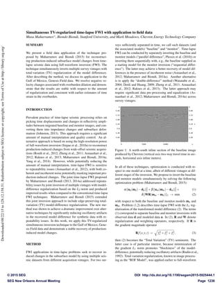
  • 1. Simultaneous TV-regularized time-lapse FWI with application to field data Musa Maharramov∗, Biondo Biondi, Stanford University, and Mark Meadows, Chevron Energy Technology Company SUMMARY We present a field data application of the technique pro- posed by Maharramov and Biondi (2015) for reconstruct- ing production-induced subsurface model changes from time- lapse seismic data using full-waveform inversion (FWI). The technique simultaneously inverts multiple survey vintages with total-variation (TV) regularization of the model differences. After describing the method, we discuss its application to the Gulf of Mexico, Genesis Field data. We resolve negative ve- locity changes associated with overburden dilation and demon- strate that the results are stable with respect to the amount of regularization and consistent with earlier estimates of time strain in the overburden. INTRODUCTION Prevalent practice of time-lapse seismic processing relies on picking time displacements and changes in reflectivity ampli- tudes between migrated baseline and monitor images, and con- verting them into impedance changes and subsurface defor- mation (Johnston, 2013). This approach requires a significant amount of manual interpretation and quality control. An al- ternative approach is based on using the high-resolution power of full-waveform inversion (Sirgue et al., 2010a) to reconstruct production-induced changes from wide-offset seismic acquisi- tions (Routh et al., 2012; Zheng et al., 2011; Asnaashari et al., 2012; Raknes et al., 2013; Maharramov and Biondi, 2014a; Yang et al., 2014). However, while potentially reducing the amount of manual interpretation, time-lapse FWI is sensitive to repeatability issues (Asnaashari et al., 2012), with both co- herent and incoherent noise potentially masking important pro- duction-induced changes. The joint time-lapse FWI proposed by Maharramov and Biondi (2013, 2014a) addressed repeata- bility issues by joint inversion of multiple vintages with model- difference regularization based on the L2-norm and produced improved results when compared to the conventional time-lapse FWI techniques. Maharramov and Biondi (2015) extended this joint inversion approach to include edge-preserving total- variation (TV) model-difference regularization. The new me- thod was shown to achieve a dramatic improvement over alter- native techniques by significantly reducing oscillatory artifacts in the recovered model difference for synthetic data with re- peatability issues. In this work, we apply this TV-regularized simultaneous inversion technique to the Gulf of Mexico, Gene- sis Field data and demonstrate a stable recovery of production- induced model changes. METHOD FWI applications in time-lapse problems seek to recover in- duced changes in the subsurface model by using multiple seis- mic datasets from different acquisition vintages. For two sur- veys sufficiently separated in time, we call such datasets (and the associated models) “baseline” and “monitor”. Time-lapse FWI can be conducted by separately inverting the baseline and monitor models (“parallel difference”, Plessix et al. (2010)) or inverting them sequentially with, e.g., the baseline supplied as a starting model for the monitor inversion (“sequential differ- ence”). The latter may achieve a better recovery of model dif- ferences in the presence of incoherent noise (Asnaashari et al., 2012; Maharramov and Biondi, 2014a). Another alternative is to apply the “double-difference” method (Watanabe et al., 2004; Denli and Huang, 2009; Zheng et al., 2011; Asnaashari et al., 2012; Raknes et al., 2013). The latter approach may require significant data pre-processing and equalization (As- naashari et al., 2012; Maharramov and Biondi, 2014a) across survey vintages. Figure 1: A north-south inline section of the baseline image produced by Chevron (vertical axis two-way travel time in sec- onds, horizontal axis inline meters). In all of these techniques, optimization is conducted with re- spect to one model at a time, albeit of different vintages at dif- ferent stages of the inversion. We propose to invert the baseline and monitor models simultaneously by solving the following optimization problem (Maharramov and Biondi, 2015): α ub(mb)−db 2 2 +β um(mm)−dm 2 2 + (1) δ WR(mm −mb) 1 → min (2) with respect to both the baseline and monitor models mb and mm. Problem (1,2) describes time-lapse FWI with the L1 reg- ularization of the transformed model difference (2). The terms (1) correspond to separate baseline and monitor inversions with observed data d and modeled data u. In (2), R and W denote regularization and weighting operators, respectively. If R is the gradient magnitude operator Rf(x,y,z) = f2 x + f2 y + f2 z , (3) then (2) becomes the “Total Variation” (TV) seminorm. The latter case is of particular interest, because minimization of the gradient L1 norm promotes “blockiness” of the model- difference, potentially reducing oscillatory artifacts (Rudin et al., 1992). Total-variation regularization, known in image process- ing as the “ROF Model”, was applied earlier to full-waveform SEG New Orleans Annual Meeting Page 1236 DOI http://dx.doi.org/10.1190/segam2015-5925444.1© 2015 SEG Downloaded08/22/15to128.12.158.51.RedistributionsubjecttoSEGlicenseorcopyright;seeTermsofUseathttp://library.seg.org/
  • 2. Application of joint TV-regularized 4D FWI inversion as a way of resolving sharp geologic boundaries (Ana- gaw and Sacchi, 2012). The solution of a large-scale opti- mization problem based on the ROF model using conventional methods is computationally challenging, prone to the “stair- casing effect” (Chambolle and Lions, 1997), and may require solution methods that involve splitting and gradient threshold- ing (Goldstein and Osher, 2009). However, time-lapse FWI appears to be a nearly ideal application for the ROF model, be- cause significant production-induced subsurface model changes are spatially bounded and have magnitudes that can be roughly estimated a priori from geomechanical and production data (Maharramov and Biondi (2014a), supplementary material). More specifically, the weighting operator W may be obtained from prior geomechanical information. For example, a rough estimate of production-induced velocity changes can be ob- tained from time shifts (Hatchell and Bourne, 2005) and used to map subsurface regions of expected production-induced per- turbation. Figure 2: Monitor and baseline image-difference obtained from the 3D time-migration images provided by Chevron and corresponding to the inline section of Figure 1. Production- induced changes stand out at approximately 3.5 s (wet Illi- noisan sands) and 4 s two-way travel times—stacked Neb 1, 2, and 3 reservoirs—compare with Hudson et al. (2005). APPLICATION TO FIELD DATA The Genesis Field, operated by Chevron, is located 150 miles southwest of New Orleans in the Green Canyon area of the central Gulf of Mexico, in approximately 770-830m of water (Magesan et al., 2005). Oil was found in several late Pliocene through early Pleistocene deep-water reservoirs. Most of the field’s oil and gas reserves are in the early Pleistocene Neb 1, Neb 2, and Neb 3 reservoirs that are the primary subject of this study. First oil production began in January 1999. A 3D seismic survey was shot in 1990, and a time-lapse survey was shot in October 2002 with the aim of improving field man- agement (Hudson et al., 2005; Magesan et al., 2005). Cumu- lative production from the field at the time of the monitor sur- vey was more than 57 MMBO, 89 MMCFG, and 19 MMBW (Hudson et al., 2005). In addition to fluid substitution effects, producing reservoirs compact, increasing the depth to the top of the reservoirs and causing overburden dilation (Johnston, 2013). A time-lapse study performed by Chevron (Hudson et al., 2005) indicated significant apparent kinematic differences in the Pleistocene reservoir interval. Time shifts were observed both for the pro- ducing reservoirs and Illinoisan wet sands above Neb 1 (see Figure 3). Kinematic differences were attributed to a time shift caused by subsidence at the top of the uppermost reservoir, subsidence of the overburden, and overburden dilation (Hud- son et al., 2005). Figure 3: Production-induced changes resulted in measurable time-shifts between the surveys. Shown here are time-shifts between the baseline (blue) and monitor (red) common-offset gathers, 1074 m offset. Parameters of the baseline and monitor surveys and subsequent time-lapse processing by Chevron were described by Magesan et al. (2005). The baseline survey had a maximum offset of 5 km, and the monitor survey had a maximum offset of 7.3 km. Both surveys had a bin size of 12.5 m by 37 m. For the purpose of time-lapse analysis, the acquired data had been sub- jected to data equalization, pre-processing and imaging steps that included a spherical divergence correction, source and re- ceiver statics, global phase rotation, time shift, amplitude scal- ing, global spectral matching, and cross-equalization (Mage- san et al., 2005). The data pre-processed for time-lapse analysis were used by Chevron in Kirchhoff time migration of the baseline and mon- itor surveys, producing 3D images. A single inline section of the baseline image is shown in Figure 1. The corresponding monitor and baseline image difference is shown in Figure 2. As noted by Hudson et al. (2005), the image difference is con- tributed to by time shifts at the Illinoisan sands (upper event) and Neb 1 (lower event) in Figure 2—compare with Figure 1 of Hudson et al. (2005). The purpose of this exercise was to verify whether or not joint regularized time-lapse FWI could resolve some of the pro- duction-induced model differences, thus providing additional insight into reservoir depletion patterns and optimal infill dril- ling strategies. As our first processing step, we performed sep- arate baseline and monitor 2D full-waveform inversion of a single inline section. We extracted a single north-south inline corresponding to the image in Figure 1 from both surveys and SEG New Orleans Annual Meeting Page 1237 DOI http://dx.doi.org/10.1190/segam2015-5925444.1© 2015 SEG Downloaded08/22/15to128.12.158.51.RedistributionsubjecttoSEGlicenseorcopyright;seeTermsofUseathttp://library.seg.org/
  • 3. Application of joint TV-regularized 4D FWI Figure 4: Inverted baseline velocity model. FWI resolved fine model features and oriented them along the dip structure of the image in Figure 1 (vertical axis depth meters). sorted it into shot gathers with a minimum offset of 350 m and a maximum offset of 4,700 m, 1,264 shots and up to 175 re- ceivers per shot. A frequency-domain 2D FWI (Sirgue et al., 2008, 2010b) was conducted over the frequency range of 3- 30.7 Hz. Frequency spacing was selected using the technique of Sirgue and Pratt (2004). The data provided to us had under- gone amplitude pre-processing that included a spherical diver- gence correction. Furthermore, accurate handling of the am- plitudes in 2D FWI of 3D field data requires a 3D-to-2D data transformation (Auer et al., 2013). Because the data exhib- ited significant time-shifts at the reservoir level (Hudson et al., 2005) that can be readily observed even at far offsets (see Fig- ure 3), we decided to use a “phase-only” inversion and ignored amplitude information in the data (Fichtner, 2011). The result of baseline inversion is shown in Figure 4. To build a starting model for the FWI, we converted Chevron’s RMS time-migration velocity model to an interval velocity using the Dix equation, and smoothed the result using a triangular filter with a 41-sample window. Observe that FWI succeeded in re- solving fine features, and oriented them consistently along the dip structure of the time-migrated image in Figure 1. Close-up views of the model area covering both the Illinoisan sands and the reservoirs are shown in Figures 6a and 6c. The result of parallel differencing is shown in Figure 5a. Al- though significant model changes appear to be concentrated around the target area, this result is not interpretable, either qualitatively or quantitatively, because it is contaminated with oscillatory artifacts and overestimates the magnitudes of ve- locity perturbations. This result is consistent with our earlier assessment of conventional time-lapse FWI techniques tested on synthetic data (Maharramov and Biondi, 2014a, 2015). Next, we solved the simultaneous, TV-regularized time-lapse full-waveform inversion problem (1,2). We set α = β = 1 and carried out multiple experiments with the value of the regular- ization parameter δ ranging from δ = 100 to δ = 1000. The weighting operator W was set to 1 inside the larger target area shown in Figures 5a through 6b, tapering off to zero outside. The results of inverting the model difference for δ = 100, 500 and 1000 are shown in Figures 5b, 5c, and 5d, respectively. Gradual increase of the regularization parameter results in the removal of most model differences with the exception of a neg- ative velocity perturbation in the overburden, peaking at ap- proximately 3.6 km and 3.9 km (see Figures 6b and 6d). Such perturbations are consistent with overburden dilation due to the compaction of stacked reservoirs, with more significant di- lation in the wet Illinoisan sands than the surrounding shales (Rickett et al., 2007). The zone of negative velocity change appears to extend upward into the overburden in a direction roughly orthogonal to the reservoir dip—see Figure 5d. Two negative velocity changes at approximately 10 and 11.5 km in- line persist with increasing regularization, and may represent dilation effects associated with the production from deeper re- servoirs—compare with Figure 3 of Rickett et al. (2007). The estimated maximum negative velocity change of −45 m/s above the stacked reservoirs is consistent with the earlier es- timates of time strain in the overburden (Rickett et al., 2007). Indeed, local time strain, physical strain and partial velocity change are related by the equation (Hatchell and Bourne, 2005) dτ dt ≈ ∆t t = ∆z z − ∆v v , (4) where τ,t,z, and v denote the observed time shift, travel time, depth, and velocity. Assuming, following Hatchell and Bourne (2005), that ∆v v = −R ∆z z , (5) where the factor R is estimated to be 6 ± 2 for the Genesis overburden (Hodgson et al., 2007), we obtain ∆v v = − R R+1 ∆t t ≈ − ∆t t ≈ − dτ dt . (6) Maximum time strains in the Genesis overburden are estimated to be around +2% (Rickett et al., 2007), yielding the maximum negative velocity change of ∆v ≈ −.02×2,800 m/s = −56 m/s, (7) where the estimated P-wave velocity of 2,800 m/s at a 3.6 km depth was taken from the output of our FWI. CONCLUSIONS Simultaneous time-lapse FWI with total-variation difference regularization can achieve robust recovery of production-in- duced changes, preserving the blocky nature of monitor-base- line differences. Velocity changes caused by overburden dila- tion are within the resolution of our method. However, veloc- ity changes within thin reservoirs (e.g., caused by compaction) can no longer be characterized as “blocky” on a seismic scale, and recovering such changes may require a multi-norm model decomposition approach a la Maharramov and Biondi (2014b), and will be the subject of further research. ACKNOWLEDGMENTS The authors would like to thank the affiliate members of Stan- ford Exploration Project (SEP) for their support; Joseph Ste- fani, Stewart Levin, Shuki Ronen, and Dimitri Bevc for a num- ber of useful discussions; Chevron for providing the field data; and the Stanford Center for Computational Earth and Environ- mental Science for providing computing resources. SEG New Orleans Annual Meeting Page 1238 DOI http://dx.doi.org/10.1190/segam2015-5925444.1© 2015 SEG Downloaded08/22/15to128.12.158.51.RedistributionsubjecttoSEGlicenseorcopyright;seeTermsofUseathttp://library.seg.org/
  • 4. Application of joint TV-regularized 4D FWI (a) (b) (c) (d) Figure 5: (a) Parallel difference and joint inversion results for (b) δ = 100, (c) δ = 500, and (d) δ = 1000 in the target area. Note that the parallel difference result is not interpretable because of the presence of artifacts. Increasing the regularization parameter δ results in gradual removal of most model differences except the negative velocity change in the overburden, peaking around the Illinoisan sands and near the top of the stacked reservoirs—see Figures 6a through 6d. (a) (b) (c) (d) Figure 6: (a) Baseline target area and (b) estimated model difference for δ = 1000. Close-up of (c) baseline target area and (b) estimated model difference for δ = 1000. SEG New Orleans Annual Meeting Page 1239 DOI http://dx.doi.org/10.1190/segam2015-5925444.1© 2015 SEG Downloaded08/22/15to128.12.158.51.RedistributionsubjecttoSEGlicenseorcopyright;seeTermsofUseathttp://library.seg.org/
  • 5. EDITED REFERENCES Note: This reference list is a copyedited version of the reference list submitted by the author. Reference lists for the 2015 SEG Technical Program Expanded Abstracts have been copyedited so that references provided with the online metadata for each paper will achieve a high degree of linking to cited sources that appear on the Web. REFERENCES Anagaw, A. Y., and M. D. Sacchi, 2012, Edge-preserving seismic imaging using the total variation method: Journal of Geophysics and Engineering, 9, no. 2, 138– 146. http://dx.doi.org/10.1088/1742-2132/9/2/138. Asnaashari, A., R. Brossier, S. Garambois, F. Audebert, P. Thore, and J. Virieux, 2012, Time-lapse imaging using regularized FWI: A robustness study: 82nd Annual International Meeting, SEG, Expanded Abstracts, doi:http://dx.doi.org/10.1190/segam2012-0699.1. Auer, L., A. M. Nuber, S. A. Greenhalgh, H. Maurer, and S. Marelli, 2013, A critical appraisal of asymptotic 3D-to-2D data transformation in full-waveform seismic crosshole tomography: Geophysics, 78, no. 6, R235–R247. http://dx.doi.org/10.1190/geo2012-0382.1. Chambolle, A., and P. L. Lions, 1997, Image recovery via total variational minimization and related problems: Numerische Mathematik, 76, no. 2, 167– 188. http://dx.doi.org/10.1007/s002110050258. Denli, H., and L. Huang, 2009, Double-difference elastic waveform tomography in the time domain: 79th Annual International Meeting, SEG, Expanded Abstracts, 2302–2306. Fichtner, A., 2011, Full-seismic modeling and inversion: Springer. http://dx.doi.org/10.1007/978-3-642- 15807-0. Goldstein, T., and S. Osher, 2009, The split Bregman method for L1-regularized problems: SIAM Journal on Imaging Sciences, 2, no. 2, 323–343. http://dx.doi.org/10.1137/080725891. Hatchell, P., and S. Bourne, 2005, Measuring reservoir compaction using time-lapse time shifts: 75th Annual International Meeting, SEG, Expanded Abstracts, 2500–2503. Hodgson, N., C. Macbeth, L. Duranti, J. Rickett, and K. Nihei, 2007, Inverting for reservoir pressure change using time-lapse time strain: Application to Genesis Field, Gulf of Mexico: The Leading Edge, 26, 649–652. http://dx.doi.org/10.1190/1.2737104. Hudson, T., B. Regel, J. Bretches, J. Rickett, B. Cerney, and P. Inderwiesen, 2005, Genesis Field, Gulf of Mexico, 4D project status and preliminary lookback: 75th Annual International Meeting, SEG, Expanded Abstracts, 2436–2439. Johnston, D., 2013, Practical applications of time-lapse seismic data: SEG. http://dx.doi.org/10.1190/1.9781560803126. Magesan, M., S. Depagne, K. Nixon, B. Regel, J. Opich, G. Rogers, and T. Hudson, 2005, Seismic processing for time-lapse study: Genesis Field, Gulf of Mexico: The Leading Edge, 24, 364– 373. http://dx.doi.org/10.1190/1.1901384. Maharramov, M., and B. Biondi, 2013, Simultaneous time-lapse full-waveform inversion: SEP Report, 150, 63–70. Maharramov, M., and B. Biondi, 2014a, Joint full-waveform inversion of time-lapse seismic data sets: 84th Annual Meeting, SEG, Expanded Abstracts, 954–959. Maharramov, M., and B. Biondi, 2014b, Multimodel full-waveform inversion: SEP Report, 155, 187– 192. SEG New Orleans Annual Meeting Page 1240 DOI http://dx.doi.org/10.1190/segam2015-5925444.1© 2015 SEG Downloaded08/22/15to128.12.158.51.RedistributionsubjecttoSEGlicenseorcopyright;seeTermsofUseathttp://library.seg.org/
  • 6. Maharramov, M., and B. Biondi, 2015, Robust simultaneous time-lapse full-waveform inversion with total-variation regularization of model difference: 77th Annual International Conference and Exhibition, EAGE, Extended Abstracts, http://dx.doi.org/10.3997/2214-4609.201413085. Plessix, R.-E., S. Michelet, H. Rynja, H. Kuehl, C. Perkins, J. W. de Maag, and P. Hatchell, 2010, Some 3D applications of full waveform inversion: Presented at the 72nd Annual International Conference and Exhibition, EAGE, Workshop WS6 3D Full-Waveform Inversion — A Game- Changing Technique?. Raknes, E., W. Weibull, and B. Arntsen, 2013, Time-lapse full-waveform inversion: Synthetic and real data examples: 83rd Annual International Meeting, SEG, Expanded Abstracts, 944–948. Rickett, J., L. Duranti, T. Hudson, B. Regel, and N. Hodgson, 2007, 4D time strain and the seismic signature of geomechanical compaction at Genesis: The Leading Edge, 26, 644–647. http://dx.doi.org/10.1190/1.2737103. Routh, P., G. Palacharla, I. Chikichev, and S. Lazaratos, 2012, Full-wavefield inversion of time-lapse data for improved imaging and reservoir characterization: 82nd Annual International Meeting, SEG, Expanded Abstracts, doi:http://dx.doi.org/10.1190/segam2012-1043.1., 1–6. Rudin, L. I., S. Osher, and E. Fatemi, 1992, Nonlinear total variation based noise removal algorithms: Physica D. Nonlinear Phenomena, 60, no. 1–4, 259–268. http://dx.doi.org/10.1016/0167- 2789(92)90242-F. Sirgue, L., O. Barkved, J. Dellinger, J. Etgen, U. Albertin, and J. Kommendal, 2010a, Full-waveform inversion: The next leap forward in imaging at Valhall: First Break, 28, no. 4, 65–70. Sirgue, L., J. T. Etgen, and U. Albertin, 2008, 3D frequency domain waveform inversion using time domain finite difference methods: 70th Annual International Conference and Exhibition, EAGE, Extended Abstracts, http://dx.doi.org/10.3997/2214-4609.20147683. Sirgue, L., J. T. Etgen, U. Albertin, and S. Brandsberg-Dahl, 2010b, System and method for 3D frequency domain waveform inversion based on 3D time-domain forward modeling: U. S. Patent 7,725,266. Sirgue, L., and R. Pratt, 2004, Efficient waveform inversion and imaging: A strategy for selecting temporal frequencies: Geophysics, 69, 231–248. http://dx.doi.org/10.1190/1.1649391. Watanabe, T., S. Shimizu, E. Asakawa, and T. Matsuoka, 2004, Differential waveform tomography for time-lapse crosswell seismic data with application to gas hydrate production monitoring: 74th Annual International Meeting, SEG, Expanded Abstracts, 2323–2326. Yang, D., A. E. Malcolm, and M. C. Fehler, 2014, Time-lapse full-waveform inversion and uncertainty analysis with different survey geometries: 76th Annual International Conference and Exhibition, EAGE, Extended Abstracts, http://dx.doi.org/10.3997/2214-4609.20141120. Zheng, Y., P. Barton, and S. Singh, 2011, Strategies for elastic full-waveform inversion of time-lapse ocean bottom cable (OBC) seismic data: 81st Annual International Meeting, SEG, Expanded Abstracts, 4195–4200. SEG New Orleans Annual Meeting Page 1241 DOI http://dx.doi.org/10.1190/segam2015-5925444.1© 2015 SEG Downloaded08/22/15to128.12.158.51.RedistributionsubjecttoSEGlicenseorcopyright;seeTermsofUseathttp://library.seg.org/