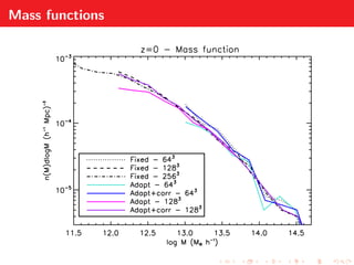
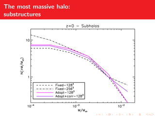
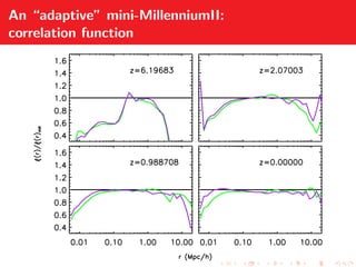
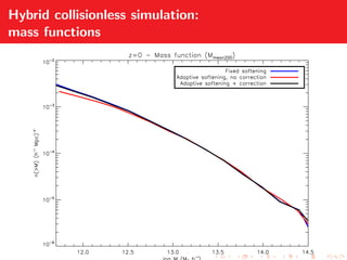
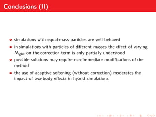
Adaptive gravitational softening allows the gravitational softening length to vary based on the local density of particles. This improves the accuracy of simulations by reducing softening in high density regions while preventing divergences in low density regions. The document discusses methods for implementing adaptive softening in cosmological simulations and hybrid simulations with particles of different masses. It also analyzes the effects of adaptive softening on mass functions, correlation functions, and the evolution of structures.

1. Adaptive gravitational softening in GADGET
Iannuzzi & Dolag (2011) and more

2. What softening is
*Monaghan & Lattanzio 1985, A&A, 149, 135

3. What we need it for
Depends on the kind of simulation one is performing:
Collisional simulation - need softening to avoid divergences and reduce
the computational time
Collisionless simulation - need softening to reduce computational time
and moderate the noise induced by the under-representation of the
particles’ DF

4. Noise vs. Bias and the optimal h
(Merritt 1996, AJ, 111, 2462)
NOISEr = (Fr − Fr )2
BIASr = Fr −Fr,true
ASEr = BIAS2
r +NOISEr = (Fr − Fr,true)2

5. Optimal h: does it always exist?

6. Adaptive softening
(Price & Monaghan 2007, MNRAS, 374, 1347)
Definition 4
3πh3ρ = mNngbs =⇒ h ∝ ρ−1/3
New Lagrangian Lgrav = N
i=1 mi
1
2v2
i − Φ (ri , h(ri ))
Equation of Motion
dvj
dt
= − G
N
i=1
mi
φij (hj ) + φij (hi )
2
rj − ri
|rj − ri |
−
G
2
N
i=1
mi
ζj
Ωj
∂Wij (hj )
∂rj
+
ζi
Ωi
∂Wij (hi )
∂rj

7. Adaptive softening
(Price & Monaghan 2007, MNRAS, 374, 1347)
Definition 4
3πh3ρ = mNngbs =⇒ h ∝ ρ−1/3
New Lagrangian Lgrav = N
i=1 mi
1
2v2
i − Φ (ri , h(ri ))
Equation of Motion
dvj
dt
= − G
N
i=1
mi
φij (hj ) + φij (hi )
2
rj − ri
|rj − ri |
−
G
2
N
i=1
mi
ζj
Ωj
∂Wij (hj )
∂rj
+
ζi
Ωi
∂Wij (hi )
∂rj

8. Adaptive softening
(Price & Monaghan 2007, MNRAS, 374, 1347)
Definition 4
3πh3ρ = mNngbs =⇒ h ∝ ρ−1/3
New Lagrangian Lgrav = N
i=1 mi
1
2v2
i − Φ (ri , h(ri ))
Equation of Motion
dvj
dt
= − G
N
i=1
mi
φij (hj ) + φij (hi )
2
rj − ri
|rj − ri |
−
G
2
N
i=1
mi
ζj
Ωj
∂Wij (hj )
∂rj
+
ζi
Ωi
∂Wij (hi )
∂rj

9. Adaptive softening
(Price & Monaghan 2007, MNRAS, 374, 1347)
Definition 4
3πh3ρ = mNngbs =⇒ h ∝ ρ−1/3
New Lagrangian Lgrav = N
i=1 mi
1
2v2
i − Φ (ri , h(ri ))
Equation of Motion
dvj
dt
= − G
N
i=1
mi
φij (hj ) + φij (hi )
2
rj − ri
|rj − ri |
−
G
2
N
i=1
mi
ζj
Ωj
∂Wij (hj )
∂rj
+
ζi
Ωi
∂Wij (hi )
∂rj

10. Adaptive softening
(Price & Monaghan 2007, MNRAS, 374, 1347)
Zeta
ζi ≡
∂hi
∂ρi
N
k=0
mk
∂φik(hi )
∂hi
Omega
Ωi ≡ 1 −
∂hi
∂ρi
N
k=0
mk
∂Wik(hi )
∂hi

11. Optimal h: fixed vs. adaptive softening

12. Correction term and energy conservation

13. Effects in a cosmological environment
No analytical solution
Keep the same power spectrum and increase the resolution
Fixed 643
Fixed 1283
Fixed 2563
Adapt 643
Adapt 1283
Adapt+corr 643
Adapt+corr 1283

14. Mass functions

15. Correlation functions

16. The most massive halo
M200 1015
M ; r200 2.4 h−1
Mpc; 3000, 21000, 160000 particles

17. The most massive halo
M200 1015
M ; r200 2.4 h−1
Mpc; 3000, 21000, 160000 particles

18. The most massive halo:
substructures

19. An “adaptive” mini-MillenniumII
low-resolution version of the MillenniumII (Boylan-Kolchin et al. 2009)
same power-spectrum, 125 times less particles
mII mini-mII
adaptive
mini-mII

20. An “adaptive” mini-MillenniumII:
mass function

21. An “adaptive” mini-MillenniumII:
correlation function

22. Conclusions (I)
adaptive softening lengths provide near-optimal softening with little
dependance on Nngbs
in order to retain energy conservation the equation of motion needs to
be modified
the use of adaptive softening in a cosmological simulation enhances
the clustering of particles at small scales, anticipating the results
obtained in higher resolution simulations

23. Hybrid simulations
Fields sampled by particles of different masses:
Collisionless species - to start with
Hydrodynamical simulations - eventually
Do we have an impact on two-body effects?

24. Hybrid collisionless simulation:
evaporation of the light component from halos

25. Hybrid collisionless simulation:
mass functions

26. Hybrid collisionless simulation:
evaporation of the light component from halos

27. Hybrid collisionless simulation:
evaporation of the light component from halos

28. Conclusions (II)
simulations with equal-mass particles are well behaved
in simulations with particles of different masses the effect of varying
Nngbs on the correction term is only partially understood
possible solutions may require non-immediate modifications of the
method
the use of adaptive softening (without correction) moderates the
impact of two-body effects in hybrid simulations

30. Distribution of the softening lengths

31. Time bins

32. Dependence on the number of neighbours
Inner density profile of a Hernquist sphere

33. Passive evolution of a bulge+halo system