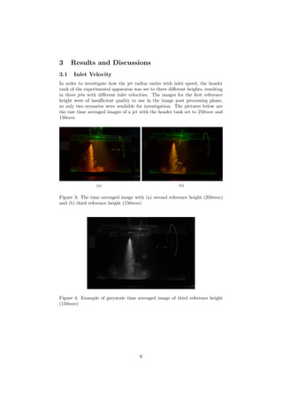
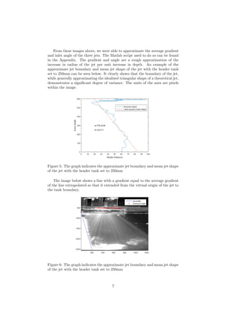
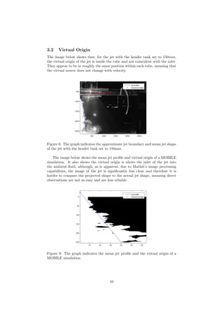
This document presents the results of an experiment and simulation investigating the properties of turbulent jets. Laser-induced fluorescence and particle image velocimetry were used to capture experimental data, while MOBILE software was used to simulate jets. Inlet velocity, virtual origin, and other properties were estimated from the experimental and simulation data using image processing and analysis in MATLAB. The results from experiment and simulation were found to correspond reasonably while some error was present.

1. Fluids 3 Coursework Report
2016
Mechanical Engineering
University of Bristol
Eugene Shing (es13906)
Robort Tanner (rt13074)
Keqin Pan (kp13594)
March 23, 2016

2. Contents
1 Introduction 3
2 Methods 4
2.1 Experimental . . . . . . . . . . . . . . . . . . . . . . . . . . . . . 4
2.1.1 Laser Induced Fluorescence . . . . . . . . . . . . . . . . . 5
2.1.2 Particle Image Velocimetry . . . . . . . . . . . . . . . . . 5
2.2 Computational . . . . . . . . . . . . . . . . . . . . . . . . . . . . 5
3 Results and Discussions 6
3.1 Inlet Velocity . . . . . . . . . . . . . . . . . . . . . . . . . . . . . 6
3.2 Virtual Origin . . . . . . . . . . . . . . . . . . . . . . . . . . . . . 10
3.3 Attenuation Constants . . . . . . . . . . . . . . . . . . . . . . . . 11
3.4 Dilution Rate . . . . . . . . . . . . . . . . . . . . . . . . . . . . . 14
3.5 Entrainment Velocity . . . . . . . . . . . . . . . . . . . . . . . . . 16
3.6 Reynold’s Number . . . . . . . . . . . . . . . . . . . . . . . . . . 18
3.7 Jet Simulation . . . . . . . . . . . . . . . . . . . . . . . . . . . . 19
4 Conclusion 22
5 Appendix 23
5.1 MOBILE input . . . . . . . . . . . . . . . . . . . . . . . . . . . . 23
5.2 The MATLAB code . . . . . . . . . . . . . . . . . . . . . . . . . 24
5.2.1 Section 3.1 - 3.2, 3.5-3.6 . . . . . . . . . . . . . . . . . . . 24
5.2.2 Section 3.3 , 3.4 . . . . . . . . . . . . . . . . . . . . . . . 27
2

3. Abstract
A moving fluids, turbulent jet entering a quiescent body of the same
fluids is modelled by both experiment and simulation. In experiment, data
is captured by camera and simulation images are produced by MOBILE.
MATLAB is used to analyse the data from experimental and simulation
in order to calculated the inlet velocity, virtual origin, attenuation con-
stant, dilution rate and Reynold’s number. The results on experimental
and simulation are shown to be corresponding to each other while some
error is present which affects the reliability of the results.
1 Introduction
Turbulent jets are fluid flows produced by a pressure drop through an orifice[1].
In this experiment, a moving fluid exits an orifice and enters a quiescent body
of the same fluid, the difference between the entering and ambient fluids create
a velocity shear which cause turbulence and mixing[2].
In this experiment, the jet formed by the Rhodamine dye solution, em-
anates from a small nozzle of width d whose axis is parallel with the z axis
which is shown in Figure 1. It then spreads out from the nozzle and forming
a well-defined boundary, which is highly turbulent in the inner layer and is
non-turbulent ambient fluid in the outer layer [3]. For the reason of flow visu-
alisation, the method of Laser Induced Fluorescence is used to investigate the
properties of the jet while the method of Particle Image Velocimetry is used to
obtain the instantaneous velocity in fluids, by adding the particles that acts as
a tracer which will glisten under laser light.
The aim of this report is to investigate the properties of turbulent jet includ-
ing virtual origin, spatial rate of dilution , entrainment velocity and Reynold’s
number and by comparing the results between the simulation, theoretical and
experimental.
Figure 1: An image illustrates the characteristic of jet [3]
3

4. 2 Methods
2.1 Experimental
There are two sections in this laboratory:
1. Laser Induced Fluorescence
2. Particle Image Velocimetry
A set of equipment is provided that is shown in Figure 1 and a Nikon cam-
era is also provided for image capturing. The tripod and the camera is first
moved to a position that is aligned with the glass tank. The camera setting is
then adjusted by varying the shutter speed, focus and ISO setting etc., in order
to capture good quality images that are suitable for analysation. The position
of the tripod and keep the camera setting is fixed once after calibration. In
this experiment, two kinds of image including instantaneous image and time-
averaged image are taken under different setting in the camera, which is 1/25”
F3.5 ISO 800 and 3” F22 ISO 400 respectively.
Experimental Equipment
Figure 2: Experimental Setup
Equipment
1 Header tank with dilute solution of Rhodamine dye
2 Jet pipe
3 Switch of laser
4 Line Laser
5 30 litre glass tank filled up with fresh water
Table 1: List of experimental equipment
4

5. 2.1.1 Laser Induced Fluorescence
The aim of this section of the experiment is to investigate the rate of intensity
decay along the ray path for a constant concentration in order to predict the
concentration when the dye is not homogenous. The procedure is listed below:
1. Adjust the height of the header tank to a known height.
2. Wiped off any gas bubbles that is presented in the glass tank.
3. Fillthe Rhodamine dye solution into the header tank and use a stopper to
restrict the flow.
4. Turn on the laser.
5. Take several instant images.
6. When the flow reaches the bottom of the glass tank, take a time averaged
image.
7. Turn off the laser.
8. Adjust the header tank to a different height and repeat the procedure
above.
2.1.2 Particle Image Velocimetry
The aim of this section is to estimate the velocity field of the horizontal entrain-
ment flow. The procedure is listed below:
1. Refill the glass tank with fresh water and flush the header tank with fresh
water in order to prevent any Rhodamine dye solution is present.
2. Particles from the demonstrator’s solution is added to the glass tank,
which will glisten in laser light.
3. Set a timer and place it beside the glass tank in order to take reference
on time.
4. Fill the header tank with fresh water and run the jet.
5. multiple images are taken with the burst mode from the camera.
2.2 Computational
MOBILE will be used to produce simulation images and the inlet velocity can be
changed in inputsetup.dat file. A modified version is attached in the Appendix.
Moreover, MATLAB will be used to process both simulation and experimental
images, the processing code is also attached in the Appendix.
5

6. 3 Results and Discussions
3.1 Inlet Velocity
In order to investigate how the jet radius varies with inlet speed, the header
tank of the experimental apparatus was set to three different heights, resulting
in three jets with different inlet velocities. The images for the first reference
height were of insufficient quality to use in the image post processing phase,
so only two scenarios were available for investigation. The pictures below are
the raw time averaged images of a jet with the header tank set to 250mm and
150mm.
(a) (b)
Figure 3: The time averaged image with (a) second reference height (250mm)
and (b) third reference height (150mm)
Figure 4: Example of greyscale time averaged image of third reference height
(150mm)
6

7. From these images above, we were able to approximate the average gradient
and inlet angle of the three jets. The Matlab script used to do so can be found
in the Appendix. The gradient and angle are a rough approximation of the
increase in radius of the jet per unit increase in depth. An example of the
approximate jet boundary and mean jet shape of the jet with the header tank
set to 250mm can be seen below. It clearly shows that the boundary of the jet,
while generally approximating the idealised triangular shape of a theoretical jet,
demonstrates a significant degree of variance. The units of the axes are pixels
within the image.
Figure 5: The graph indicates the approximate jet boundary and mean jet shape
of the jet with the header tank set to 250mm
The image below shows a line with a gradient equal to the average gradient
of the line extrapolated so that it extended from the virtual origin of the jet to
the tank boundary.
Figure 6: The graph indicates the approximate jet boundary and mean jet shape
of the jet with the header tank set to 250mm
7

8. The inlet velocity of each jet was first estimated using Bernoulli’s equation,
assuming that the fluid in the header tank was at rest and hydrostatic pressure
was constant throughout the jet system, the initial estimate of inlet velocity, v0,
was therefore:
v0 = 2gh (1)
Where h is the height of the header tank above the main tank, and g is
acceleration due to gravity. However, this estimate was inadequate, as it did
not account for friction losses in the tube. Therefore, the approximation of the
inlet velocity was improved by first calculating the Reynold’s number of the flow
through the tube. From this, and the relative roughness of the tube, and using
a Moody solver, a better estimate was found, accounting for losses in speed due
to friction. The inlet velocity, calculated as a function of the Darcy friction
factor is:
u =
2r
ρfL
∆P (2)
Where r is the radius of the tube, ∆P is the pressure drop across the tube, f
is the Darcy friction factor, ρ is the density of the Rhodamine solution and L
is the length of the tube.
The estimate of the inlet velocity was improved in an iterative process until
the solutions converged on a single result. The results are tabulated below.
Tank Height(mm) Inlet Velocity(m/s) Gradient Inlet Angle(◦
)
150 0.34 −6.73 8.45
250 0.44 −9.21 6.13
Table 2: It shows the estimated inlet velocity and angle from experimental data.
8

9. Several examples of jet simulations with a characteristic size of 128 produced
by MOBILE are shown below. In each simulation the inlet velocity is different
and the jet has become fully evolved and has just reached the ”floor” of the
simulation. They shows that faster jets are generally narrower.
(a) (b) (c)
Figure 7: The simulation images with inlet velocity (a) 0.2ms−1
and (b)
0.4ms−1
and (c) 1.0ms−1
Image Inlet Velocity (m/s) Gradient Inlet Angle (◦
)
a 0.2 −5.2 11
b 0.4 −6.2 9.2
c 1.0 −7.8 7.3
Table 3: It shows the estimated inlet angle from simulation data.
The table below combined both experimental and simulation results to-
gether.
Data Inlet Velocity (m/s) Gradient Inlet Angle (◦
)
Simulation 0.2 −5.2 11
Experiment 0.34 −6.73 8.45
Simulation 0.4 −6.2 9.2
Experiment 0.44 −9.21 6.13
Simulation 1.0 −7.8 7.3
Table 4: It shows the estimated inlet angle from simulation data.
It can observed that errors are presented from the experimental data accord-
ing to the trend in the inlet angle, the values highlighted in red are expected to
be larger.
9

10. 3.2 Virtual Origin
The image below shows that, for the jet with the header tank set to 150mm,
the virtual origin of the jet is inside the tube and not coincident with the inlet.
They appear to be in roughly the same position within each tube, meaning that
the virtual source does not change with velocity.
Figure 8: The graph indicates the approximate jet boundary and mean jet shape
of the jet with the header tank set to 150mm
The image below shows the mean jet profile and virtual origin of a MOBILE
simulation. It also shows the virtual origin is above the inlet of the jet into
the ambient fluid, although, as is apparent, due to Matlab’s image processing
capabilities, the image of the jet is significantly less clear and therefore it is
harder to compare the projected shape to the actual jet shape, meaning direct
observations are not as easy and are less reliable.
Figure 9: The graph indicates the mean jet profile and the virtual origin of a
MOBILE simulation
10

11. In the experimental setup, the inlet nozzle of the jet is not illuminated by
the laser due to the fan-shaped laser profile. However, the nozzle does not need
to be illuminated as the jet is sufficiently self-similar for most of its length that
a mean profile can be determined and, through a simple process of linear re-
gression, the approximate location of the virtual source can be identified.
We are fairly confident that the approximation to the virtual source is ac-
curate, as the jet profiles extending from the virtual sources found by linear
regression follow the shape of the experimental jet closely.
3.3 Attenuation Constants
In the experiment, several images of different Rhodamine dye concentration so-
lution are processed in MATLAB in order to determine the relationship between
light intensity and concentration. The images are first converted into greyscale
and the light intensity is normalised as 1.0 to make a better comparison. By
reducing the error caused by the reflection of light from surrounding, the result
from multiple rays is averaged. Therefore, according to the Lambert Beer’s Law,
∂I
∂s
= −ηI (3)
Where I represents the intensity of the light ray, η represents the attenuation
rate.
The intensity can be updated on a given ray by:
Ik+1 = Ikeηs
(4)
where k and k + 1 are the position of the ray.
In this experiment, the model of η is linear:
η = aC + b (5)
where C represents the dye concentration, a is the constant for attenuation co-
efficient and b is the constant for background level attenuation.
To construct a linear relationship equation, taking natural logarithm on both
side in equation 4 and let k = 0, which will get:
ln(I1) = ln(I0) − ηs (6)
A graph is then plot by MATLAB which is shown in below and by calculating
the gradient, the attenuation constants can be found.
11

12. Figure 10: Relationship between ln(Intensity) against distance with different
concentrations
Concentration η(molm−3
)
C1 4.25 × 10−3
C2 4.06 × 10−3
C3 4.01 × 10−3
Table 5: It shows the attenuation rate with different concentration
Assuming C1 = C, C2 = 2C and C3 = 3C, since there are two unknowns
in total, only two set of data are needed. However, in order to obtain better
accuracy of results, a graph of attenuation rate against concentration is plotted
with all three sets of data and by plotting the best-fit line, the value of aC and
b can be estimated.
Figure 11: Relationship between attenuation rate against concentration
From Figure 11, aC is calculated as −1.00×10−4
by calculating the gradient
and by finding the y-interception, b is found as 4.30 × 10−4
.
Since the value of a is still undefined, it is important to understand the
relationship between aC against the distance along the ray, which is shown in
Figure 12. A mean value of aC is also plotted for comparison.
12

13. Figure 12: Relationship between aC against distance with different concentra-
tions
It can be observed that although small fluctuations occur in all the diagrams
above, the values are closed to the mean values that are plotted in red. This can
be explained the concentration remains constant throughout the experiment. As
a result, it is not required to know a independently.
13

14. 3.4 Dilution Rate
When the jet in term of Rhodamine dye solution gets into the glass tank, the
concentration of jet will be diluted as the jet get further away from nozzle be-
cause the jet is engulfed by the surrounding fluid. Conversion between light
intensity and concentration is made from the experimental results according to
the Lambert Beer Law:
e−(aC+b)s
=
I
Imax
(7)
With a and b are calculated above, the graphs of dilution rate from simu-
lation and experiment are plotted under different inlet velocities are shown in
Figure 13 and 14. It can be observed that the simulation graph fluctuated more
rapidly as the contrast of the images are sharper.
(a) (b)
Figure 13: The dilution rate of centre jet for 0.34ms−1
(a) from simulation (b)
from experiment
(a) (b)
Figure 14: The dilution rate of centre jet for 0.44ms−1
(a) from simulation (b)
from experiment
The difference between the simulation and experimental results can be ex-
plained by noise that existed in the experimental image.
14

15. Figure 15 and 16 shows the concentration field from simulation and exper-
iment. From the graphs, the dye diffuses sharply when it is closer to bottom
of tank and concentration of jet decreases as it moves downward. It is worth
noting that from the experiment graph, the peak is narrower because of the
small size of nozzle in the experiment setup.
(a) (b)
Figure 15: The concentration field for 0.34ms−1
(a) from simulation (b) from
experiment
(a) (b)
Figure 16: The concentration field for 0.44ms−1
(a) from simulation (b) from
experiment
Figure 17 shows jet and laser ray from simulation. Since the dye absorbed
light, its intensity decreases significantly when light passing through. From the
left hand side of the graph, since the jet is closer to the laser, the light intensity
is higher than the right hand side. Moreover, according to Lambert Beer’s law,
light intensity will decrease as concentration increases which is shown in the
right hand side of the graph, where the light intensity decreased. Therefore, it
can be proved that the light intensity field is not identical with the concentration
field.
15

16. Figure 17: Graph indicates the jet and the position of the laser ray
3.5 Entrainment Velocity
Using the two images show below, the entrainment velocity field of the jet was
estimated.
Figure 18: The two instant images that show the movement of particle.
The images were read into Matlab and all colours of light besides green were
screened out, as the green-coloured illuminated particles were the significant
data. A small region 700 x 700 pixels in size just to the right of the jet was iso-
lated. Then, counting from the centre of that region, it was estimated that tiles
100 x 100 pixels in size would each contain roughly thirty particles, assuming a
homogenous distribution throughout the fluid.
The small section of image was broken into forty-nine tiles, each 100 x 100
pixels in size. Once the corresponding tiles for the two different timestamps
were cross-correlated and the required displacement vectors found, they were
converted to velocity vectors using the scale and time difference between the
images.
The image below is an approximation of the entrainment velocity field be-
tween the two images of the jet and illuminated particles. There is a certain
degree of statistical noise in the results. This is likely due to the possibility
that some tiles had a fewer number of particles than the required thirty or
16

17. possibly due to poor illumination, in some tiles it is very possible that the par-
ticles observed had entered into or left the illuminated plane between time-steps.
The average magnitude of the entrainment velocity is approximately 0.4mms−1
.
Figure 19: The graph indicates the approximation of the entrainment velocity
field between the two images of the jet and illuminated particles.
The image below is the horizontal (x-direction) velocity field of a MOBILE
simulation of a jet. It shows that the velocity field in the ambient fluid, and
therefore the entrainment velocity, is homogenous and apparently constant.
Figure 20: Horizontal velocity field from simulation
Theoretically the entrainment velocity of the jet should vary with depth, as
it is proportional to the axial speed, which decreases as the jet spreads through
the ambient fluid. This is not observed in the experiment or the MOBILE simu-
lation, presumably because the PIV and MOBILE models only observe a small
section of a jet, and the small change in depth means that a significant change
in entrainment speed would not be observed.
17

18. 3.6 Reynold’s Number
The Reynolds number can be calculated using the density and kinematic vis-
cosity of the Rhodamine dye solution, and a turbulent length scale and velocity
scale. Assuming that the Rhodamine dye is sufficiently diluted that it has the
density and kinematic viscosity of water, and taking the length scale as the
radius of the jet and the axial speed of the jet as the speed scales, then the
Reynolds number at the inlet can be calculated as:
Re =
ρuL
µ
=
1000 × 0.394 × 0.004
0.001
= 1574.4 (8)
The Reynolds number of the jet should remain constant throughout the jet,
assuming that the jet is self-similar.
The plots below show the concentration profile and normalised concentra-
tion profiles at various depths within the jets. They appear to approximate a
Gaussian function, and the normalised profiles appear to be sufficiently similar
that self-similarity is a reasonable assumption.
Figure 21: The graph indicates the concentration profile
18

19. Figure 22: The graph indicates the normalised concentration profile
3.7 Jet Simulation
Using the information gathered in this experiment, as well as skills gained
throughout the course, a rudimentary simulation of a turbulent jet. This simu-
lation does not have the power and resolution available to MOBILE, nor can it
model the effect of turbulent eddies or of the jet impacting a solid surface.
The jet was modelled by discretising the turbulent diffusion equation:
∂ϕ
∂t
=
1
r
∂
∂r
κr
∂ϕ
∂r
(9)
Where ϕ is the concentration of the dye, r is the radius of the jet and κ is the
diffusion coefficient, calculated as:
κ = γur (10)
Where γ is a scalar constant and u is the axial speed of the jet. In this sim-
ulation, the time derivative was first converted to a spatial derivative, so each
time step was assumed to be equivalent to one step along the centreline of the jet.
∂ϕ
∂t (n+ 1
2 )∆t
=
dz
dt
∂ϕ
∂z
= u
∂ϕ
∂z
= un
i
ϕn+1
− ϕn
i
∆z
(11)
The spatial derivative at distance from the centreline of the jet can be ap-
proximated as:
r
∂
∂r
r
∂ϕ
∂r i∆r
=
r∂ϕ
∂r
(i+ 1
2 )∆r
− r∂ϕ
∂r
(i− 1
2 )∆r
∆r
(12)
19

20. This expression simplifies to:
ri+ 1
2
ϕn
i+1 − ri+ 1
2
+ ri− 1
2
ϕn
i + ri− 1
2
ϕn
i−1
(∆r)2
(13)
And, since:
ri+ 1
2
= r +
∆r
2
, ri− 1
2
= r −
∆r
2
(14)
Therefore:
ϕn+1
i = ϕn
i +
κ(∆z)
unri(∆r)2
ri+ 1
2
ϕn
i+1 − 2riϕn
i + ri− 1
2
ϕn
i−1 (15)
The stability criterion of the discretised expression was found by setting the
value of to and all other values to zero. Applying these conditions to the dis-
cretised equation produced the value:
ϕn+1
i = ε 1 −
2κ(∆z)
unri(∆r)2
(16)
For the calculation to be stable, the error must remain constant or decay between
time-steps, and, in order to prevent further instability, the error must not change
sign between time-steps. Applying these conditions to the error expression
results in the final stability criterion for the simulation:
∆z
(∆r)2
<
un
ri
2κ
(17)
∆z
(∆r)2
<
1
2γ
(18)
As γ is a constant, in order to ensure stability, ∆z must be significantly less
than ∆r . In the jet simulation, the value of ∆z was set to 0.1, and ∆r to 1.
After a series of trial-and-error, γ was set to 0.1.
The simulation modelled only the right-hand side of the jet, as the jet was
assumed to be axisymmetric. Since modelling from a point source would have
been difficult, the Matlab simulation was designed to model from the outlet of
the tube.
For each time-step, the newly generated row in the matrix was extracted
and all values divided by the maximum value, producing row vector represent-
ing the normalised concentration field, ϕ (r). The discrete approximation to
the cumulative distribution function of the normalised concentration field,ψ(r),
was found by taking the cumulative sum of the row vector, and the maximum
value,ψ(∞), was extracted. Using these values, an approximation to the jet ra-
dius was calculated and recorded in a storage vector. The plot below shows the
evolution of the radius with depth of the jet in the simulation, and it appears to
show the transition from a cylindrical to conical profile, as predicted by theory
and observed in the MOBILE simulations.
20

21. Figure 23: The graph indicates the relationship between the radius and depth
of the jet in the simulation.
The mass flow rates through each face were calculated, and the entrainment
speed was calculated as the difference between them divided by the lateral
surface area of the control volume. The rate of change of the mass flow rate
between each face was used to find the entrainment coefficient. The plot below
shows the evolution of the axial and entrainment speeds of the jet. The axial
and entrainment speeds both clearly decrease with time, which supports the
theory that there is some relationship between them. Also, the entrainment
coefficient appears to increases exponentially, which is also understandable, as
the jet spreads out, a greater amount of fluid must be entrained into the jet,
and the entrainment coefficient therefore increases.
Figure 24: The graph indicates the evolution of the axial and entrainment speeds
of the jet
21

22. 4 Conclusion
The main objective of this investigation in this report is to compare the dif-
ferences between the theoretical results and the simulation and experimental
results under different aspects, including the inlet velocity, spread rate, virtual
origin, dilution rate and the entrainment velocity.
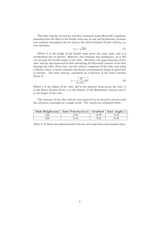
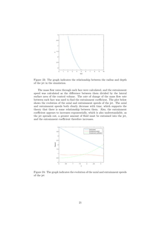
For the inlet velocity, it can be proved that both experimental and simula-
tion data shows the trend that a faster jets will give a smaller inlet angle. Some
error can be observed as the experimental data is expected to be larger.
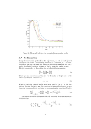
The MOBILE simulations and experimental observations for the virtual ori-
gin appear to support one another and it also proved that the virtual source does
not change with velocity. However, ”truncation error” is present as the standard
iterative process used to solve parabolic equations relies on Taylor expansions of
differential equations, and frequently discount any terms of third order or higher.
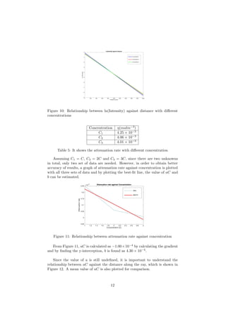
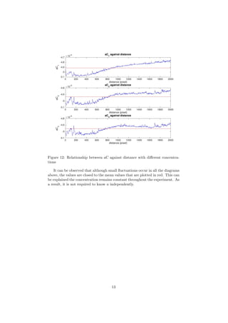
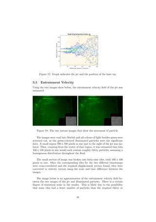
Attenuation constant can be found according to Lambert Beer’s law. It
is found that the maximum error between the aC value to the mean value is
about 3.30%. Therefore, it is not required to know a independently as the error
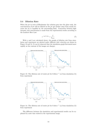
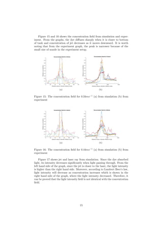
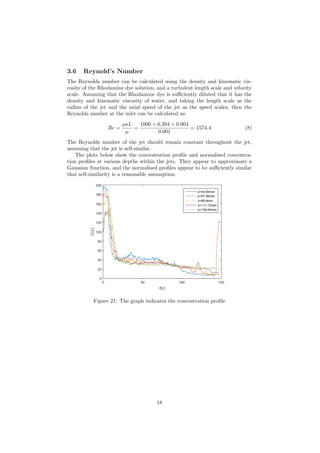
is small. Moreover, both experimental and simulation results in dilution rate
are similar. However, because of the size of the nozzle, the peak value of the
graph from the experimental results appear to be sharper.
Particle Image Velocimetry is the method used to analysis the entrainment
velocity. However, due to certain degree of statistical noise in the results, which
makes the results are not reliable enough.
In conclusion, it shows that both simulation data and experimental data
support each other. However, apart from the truncation error mentioned above,
the error that existed in the experimental data can be explained by the poor
quality of image, human error in experiment and noise existed in the image. To
improve this, some opaque plastic sheet can be placed beside the glass tank to
avoid noise from the surrounding and nevertheless, ensure the gas bubbles are
wiped off from the glass tank in order to improve the quality of image.
References
[1] E. J .List, 1982 Turbulent Jets And Plumes [Online], California Institute of
Technology
Available from: http://www.annualreviews.org/doi/pdf/10.1146/
annurev.fl.14.010182.001201 [Accessed 21st March 2016]
[2] Cushman-Roisin, B.C.R. , 2014 Environmental Fluid Mechanics [Online],
Thayer School of Engineering, Dartmouth College
Available from: https://engineering.dartmouth.edu/~d30345d/books/
EFM/chap9.pdf [Accessed 21st March 2016]
22

23. [3] Lawrie, A.G.W, 2016 Submerged Turbulent Jet [Online], University of
Bristol
Available from: https://www.ole.bris.ac.uk/bbcswebdav/
pid-2395821-dt-content-rid-6510483_2/courses/MENG30001_2015/
jet_similarity%282%29.pdf [Accessed 21st March 2016]
5 Appendix
5.1 MOBILE input
begin();
usempi:=assign(ON);
igmx:=assign(2);
jgmx:=assign(igmx);
kgmx:=assign(igmx*2);
tnx:=assign(256);
tny:=assign(tnx);
tnz:=assign(tnx*2);
xmax:=assign(1.0);
ymax:=assign(xmax);
zmax:=assign(xmax*2);
mgrids:=assign(7);
cgrids:=assign(1);
scorder:=assign(LONEDENSITY);
hsorder:=assign(SECOND);
nscalars:=assign(2);
nheights:=assign(4);
writestrat:=assign(OFF);
writescalars:=assign(OFF);
#istop:=assign(20);
iprint:=assign(1000);
#tprint:=assign(0.50);
tstop:=assign(200);
tderive:=assign(0.25);
#iderive:=assign(180);
postmem:=assign(DYNAMIC);
dtmod:=assign(OFF);
divtol:=assign(2.4e-2);
petol:=assign(1e-4);
pdtol:=assign(1e-12);
pctol:=assign(1e-12);
#
topbc:=assign(FORCEDINFLOW);
botbc:=assign(INDUCEDOUTFLOW);
leftbc:=assign(SLIPWALL);
rightbc:=assign(SLIPWALL);
frontbc:=assign(SLIPWALL);
backbc:=assign(SLIPWALL);
bcprofile:=assign(TOPHAT);
23

24. writebounds:=assign(ON);
writebcprofile:=assign(ON);
writeppert:=assign(OFF);
readppert:=assign(OFF);
bcbaseflow:=assign(-0.4);
writebcmean:=assign(ON);
bcturbamp:=assign(0.0);
bcturbvel:=assign(0.0);
bccoflowvel:=assign(0.0);
bccoflowrad:=assign(0.05);
#
#readchkfile:=assign(ON);
#istart:=assign(100);
#tstart:=assign(9.091178);
tlimit:=assign(4);
readtlimfile:=assign(ON);
end();
5.2 The MATLAB code
5.2.1 Section 3.1 - 3.2, 3.5-3.6
function timeaverage2(list)
%demonstration of time−average processing
nfiles=size(list); %find the size of the list passed in
nfiles=nfiles(2); % assumes 2D matrix, so take second element
for i=1:nfiles
%this will need editing for simulation data
infile=sprintf('DSC %04d.JPG',list(i));
outfile=sprintf('bw %04d.bmp',list(i));
imdata=imread(infile); % read image from file
% image(imdata); % output image to screen
imdata=double(imdata);
sz=size(imdata); % find the size of the image
imbw=zeros(sz(1),sz(2)); % set up a new B&W image array of the same size
imbw=sqrt((imdata(:,:,1).*imdata(:,:,1))+(imdata(:,:,2).*imdata(:,:,2))+(imdata(:,:,3).*imdata(:,:,
mx=max(max(imbw)); %find max value
mn=min(min(imbw)); %find min value
if (mx−mn)>0 %protect in case image is all zeros
imbw=(imbw−mn)/(mx−mn); %normalise to [0,1]
end
% image(imbw) %plot the scalar image in matlab colour scheme
if i==1
immean=imbw; % initialise the cumulative count to zero
else
immean=immean+imbw; %add one image each time.
end
immono=zeros(sz(1),sz(2),3);
immono(:,:,1)=imbw; %use the same value for Red
immono(:,:,2)=imbw; % Green
immono(:,:,3)=imbw; % Blue
imwrite(immono,outfile,'bmp'); %write out new greyscale file
% image(immono)
end
immean=immean/nfiles; %take the average intensity (outside the loop)
24

25. % image(immean); %plot the mean scalar... x256?
imwrite(immean,'exp mean.bmp','bmp');
% Constrain to lluminated half of the jet
% Remember that columns are x−coordinates and rows are y
immean=immean(1:2570,1800:3030);
% Use this image to create background image for shape plot
imwrite(immean,'background.png','png')
% Proces time−average image
clc
sz=size(immean);
% image(immean)
%smooth field before plotting the intensity gradient
nx=sz(1);
ny=sz(2);
%elliptic smoothing to get rid of pixel−frequency noise
for it=1:10
for ix=2:nx−1
for iy=2:ny−1
immean(ix,iy)=0.25*(immean(ix+1,iy)+immean(ix,iy+1)+immean(ix−1,iy)+immean(ix,iy−1));
end
end
end
imdx=immean(2:nx,2:ny)−immean(1:nx−1,2:ny); %divided by dx...
imdy=immean(2:nx,2:ny)−immean(2:nx,1:ny−1); %divided by dy...
imgrad=imdx.*imdx+imdy.*imdy;
% image(imgrad)
% Constrain to small section of jet
imgrad=imgrad(930:1530,25:225);
% Due to flip from image space to matrix space
% To get matrix that represents image in cartesian coordinates
imgrad=imgrad.';
sz=size(imgrad);
nx=sz(1);
ny=sz(2);
% image(imgrad)
%create an index field
xindex=zeros(nx,ny);
for ix=1:nx
for iy=1:ny
xindex(ix,iy)=ix;
end
end
%find the (normalised) moment
xmoment=zeros(1,ny);
for iy=1:ny
num=sum(imgrad(:,iy).*xindex(:,iy));
den=sum(imgrad(:,iy));
xmoment(iy)=num/den;
end
figure(1);
yidx=ny:−1:1;
plot(xmoment,yidx);
% Find a and b using matrix algebra
25

26. X=[ones(1,ny); xmoment]';
Y=yidx';
A1=(X'*Y);
A2=(X'*X);
A=inv(A2)*A1;
hold on
b=A(2,1);
a=A(1,1);
xfit=((yidx−a)/b);
plot(xfit,yidx);
axis([0 100 0 600])
legend('Actual jet shape','Least−squares mean shape')
xlabel('Axial depth')
ylabel('Radial distance')
text(20,300,['a=',num2str(a)])
text(20,250,['b=',num2str(b)])
figure(2);
background=imread('background.png');
image(background)
colormap(gray)
% Converting back to image space
X=[0:1:200];
X0=1;
X1=X−24;
hold on
d=−b;
c=930;
Y=c+(d*X1);
Y0=Y(1,1);
theta=atan(200/(2570−Y0));
thetad=theta*(180/pi);
plot(X,Y,'−b',X0,Y0,'or')
legend('Jet profile','Virtual jet origin')
text(300,500,['Jet angle is ',num2str(thetad),' degrees'],'color','red')
% Isolate an image of just the right hand side of the jet
immean2=imread('exp mean.bmp');
immean2=double(immean2);
immean2=immean2(709:2570,1800:3030);
sz=size(immean2);
% Find five depths within the jet
dz=sz(1)/10;
xmax=sz(2);
Z=round([2*dz 3*dz 4*dz 5*dz 6*dz]);
X2=[1:1:xmax];
% 2090 pixels = 250 mm
% 1 pixel = 0.12 mm
D=Z*0.12;
RZ=X2*0.12;
26

27. % Take five slices out of the concentration field
C1=immean2(Z(1,1),:);
C2=immean2(Z(1,2),:);
C3=immean2(Z(1,3),:);
C4=immean2(Z(1,4),:);
C5=immean2(Z(1,5),:);
% Plot concentration profiles
figure(3)
plot(RZ,C1,RZ,C2,RZ,C3,RZ,C4,RZ,C5)
legend(['z=',num2str(D(1,1)),'mm'],['z=',num2str(D(1,2)),'mm'],...
['z=',num2str(D(1,3)),'mm'],['z=',num2str(D(1,4)),'mm'],...
['z=',num2str(D(1,5)),'mm'])
xlabel('r(z)')
ylabel('C(z)')
% Estimate radii
R=D*tan(theta);
% Normalise concentration profiles to check for similarity
RN1=RZ/R(1,1);
RN2=RZ/R(1,2);
RN3=RZ/R(1,3);
RN4=RZ/R(1,4);
RN5=RZ/R(1,5);
CN1=C1/max(C1);
CN2=C2/max(C2);
CN3=C3/max(C3);
CN4=C4/max(C4);
CN5=C5/max(C5);
figure(4)
plot(RN1,CN1,RN2,CN2,RN3,CN3,RN4,CN4,RN5,CN5)
legend(['z=',num2str(D(1,1)),'mm'],['z=',num2str(D(1,2)),'mm'],...
['z=',num2str(D(1,3)),'mm'],['z=',num2str(D(1,4)),'mm'],...
['z=',num2str(D(1,5)),'mm'])
axis([0 1 0 1])
xlabel('r(z)/r')
ylabel('C(z)/C0')
end
5.2.2 Section 3.3 , 3.4
function attenuation()
clc
clear
filemin=1; %put your own favourite file number in here
filemax=3;
ifile=0;
xlaser=32; %source position
zlaser=0; %source position
divergence=120; %spread angle of laser sheet
nrays=121; %refinement of ray casting
raylength=2000; %how many increments along ray
dzray=1; % vertical increment of ray on grid
a=−0.0001; %attenuation cofficient proportional to concentration
b=−0.00043; %background level of attenuation
27

28. for i=filemin:filemax
filename=sprintf('%d.jpg',i);
if (exist(filename)==2)
ifile=ifile+1;
%This i s where the hard work b e gi n s
scal=imread(filename); % read image
% scal=double(scal);
% scal=scal(:,:,1); %greyscale, so take only one component
scal=double(scal(393:2392,433:3761,1));
%scal=uint8(scal);
%imshow(scal)
scal=scal/256;
% image(scal*256); %needs range 0<p<256 to plot picture
scal=scal'; %x is now horizontal, z vertical
% scal(:,:)=0.0;
% scal(32:96,:)=1.0;
%create array for light ray positions
aray=(−divergence/2:divergence/2)*pi/180; %angle of ray
dxray=dzray*tan(aray); %the dx across for each dz down
xray=zeros(raylength,nrays); %position of ray
zray=zeros(raylength,nrays); %position of ray
pray=zeros(raylength,nrays); %intensity of ray
xdom=size(scal);
xdom=xdom(1);
xray(1,:)=xlaser; %initial position
zray(1,:)=zlaser;
pray(1,:)=1.0;%normalised intensity
%%%%%
%following each ray along its length
for ir=2:raylength
%update the current x and z positions
xray(ir,:)=xray(ir−1,:)+dxray(1,:);
zray(ir,:)=zray(ir−1,:)+dzray;
%stop rays running of the left and right edges of the domain
for jr=1:nrays
if xray(ir,jr) < 3
xray(ir,jr)=3;
end
if xray(ir,jr) > xdom−2
xray(ir,jr)=xdom−2;
end
end
%during the descent by dzray the most extreme ray at 60 degrees
%could at most traverse three square cells (tan?−1 2 = 63 deg)
xf=int16(floor(xray(ir,:))); %decide which cell ray leaves from
xfm=int16(floor(xray(ir−1,:))); %decide which cell ray arrives
for jr=1:nrays %stop rays running off the edge
if xf(jr) < 3
xf(jr)=3;
end
if xf(jr) > xdom−2
xf(ix)=xdom−2;
end
if xfm(jr) < 3
28

29. xfm(jr)=3;
end
if xfm(jr) > xdom−2
xfm(jr)=xdom−2;
end
end
divsin=sin(aray);
divsin=1.0./divsin;
ltmp=sqrt(dxray.*dxray+dzray*dzray);
ptmp=pray(ir−1,:);
conc=scal(:,ir−1);
conc=conc';
%eta=(a*conc(xf)+b);
%ptmp=ptmp.*exp(−eta.*ltmp);
%work out geometry of face−crossings
for jr=1:nrays
if xf(jr)−xfm(jr) == 0 %crosses no faces (one cell only)
eta=(a*conc(xf(jr))+b); %use calibration to calculate attenuation rate
ptmp(jr)=ptmp(jr)*exp(−eta*ltmp(jr)); %exponential decay of intensity
end
if xf(jr)−xfm(jr) == 1 %crosses one face to the right
ltmp1= (double(xf(jr))−xray(ir−1,jr))*divsin(jr); %hypotenuse
eta=(a*conc(xfm(jr))+b);
ptmp(jr)=ptmp(jr)*exp(−eta*ltmp1);
ltmp2= ltmp(jr)−ltmp1;
eta=(a*conc(xfm(jr)+1)+b);
ptmp(jr)=ptmp(jr)*exp(−eta*ltmp2);
end
if xf(jr)−xfm(jr) == 2 %crosses two faces to the right
ltmp1= (double(xf(jr))−1−xray(ir−1,jr))*divsin(jr);
eta=(a*conc(xfm(jr))+b);
ptmp(jr)=ptmp(jr)*exp(−eta*ltmp1);
ltmp2= (double(xf(jr))−xray(ir−1,jr))*divsin(jr);
ltmp2= ltmp2−ltmp1;
eta=(a*conc(xfm(jr)+1)+b);
ptmp(jr)=ptmp(jr)*exp(−eta*ltmp2);
ltmp3= ltmp(jr)−ltmp1−ltmp2;
eta=(a*conc(xfm(jr)+2)+b);
ptmp(jr)=ptmp(jr)*exp(−eta*ltmp3);
end
if xf(jr)−xfm(jr) == −1 % crosses one face to the left
ltmp1= (xray(ir−1,jr)−double(xfm(jr)))*divsin(jr);
eta=(a*conc(xfm(jr))+b);
ptmp(jr)=ptmp(jr)*exp(−eta*ltmp1);
ltmp2= ltmp(jr)−ltmp1;
eta=(a*conc(xfm(jr)−1)+b);
ptmp(jr)=ptmp(jr)*exp(−eta*ltmp2);
end
if xf(jr)−xfm(jr) == −2 % crosses two faces to the left
ltmp1= (xray(ir−1,jr)−double(xfm(jr)))*divsin(jr);
eta=(a*conc(xfm(jr))+b);
ptmp(jr)=ptmp(jr)*exp(−eta*ltmp1);
ltmp2= (xray(ir−1,jr)−double(xfm(jr)+1))*divsin(jr);
ltmp2= ltmp(jr)−ltmp1;
eta=(a*conc(xfm(jr)−1)+b);
ptmp(jr)=ptmp(jr)*exp(−eta*ltmp2);
ltmp3= ltmp(jr)−ltmp1−ltmp2;
eta=(a*conc(xfm(jr)−2)+b);
ptmp(jr)=ptmp(jr)*exp(−eta*ltmp3);
end
end
29

30. pray(ir,:)=ptmp; %update final intensity array
end
figure (1)
contour(zray,xray,pray);
contour(scal);
pray mean(i,:)=mean(pray,2); % separate three intensity
%section 3.4 dilution rate
% figure(2)
% contour(zray,xray,pray,100);
% hold on
% contour(scal);
% hold off
% title('Graph of jet and position of laser ray')
% xlabel('Distance jet travels in z direction')
% ylabel('Radius of jet in x direcion')
% set(gcf,'color','white');
end
end
%section 3.3
% Attenuation constant
%%%%%%%%%%%%%%%%%%%%%%%%%%%%%%%%%%%
figure(1)
s=[1:2000];
s=s';
%1st
y1=(pray mean(1,:))';
%2nd
y2=(pray mean(2,:))';
%3rd
y3=(pray mean(3,:))';
%taking natural log to the intensity
y1=log(y1);
y2=log(y2);
y3=log(y3);
%plotting graph from the raw data
figure (1)
f1= plot(s,y1,'b','LineWidth', 2);
f1 r= get(f1,'YData');
hold on
f2=plot(s,y2,'r','LineWidth', 2);
f2 r= get(f2,'YData');
f3= plot(s,y3,'g','LineWidth', 2);
f3 r= get(f3,'YData');
title('raw')
%plotting graph for the best fit
figure (2)
p=polyfit(s,y1,1);
f1 = polyval(p,s);
plot(s,f1,'b','LineWidth', 2)
hold on
p2=polyfit(s,y2,1);
f2 = polyval(p2,s);
plot(s,f2,'r','LineWidth', 2)
p3=polyfit(s,y3,1);
f3 = polyval(p3,s);
plot(s,f3,'g','LineWidth', 2)
xlabel('Distance (pixel)')
30

31. ylabel('In (Intensity)')
title('In(Intensity) against distance')
% plotting the aC against distance, to show small fluctuation of the
% graphs
figure (3)
f1 diff=diff(f1 r);
f2 diff=diff(f2 r);
f3 diff=diff(f3 r);
s=[1:1999];
s=s';
subplot(3,1,1)
plot(s,f1 diff,'b')
hold on
f1 dmean 1=mean(f1 diff)
f1 dmean=zeros(size(s'));
f1 dmean(1,:)=f1 dmean 1;
plot(s,f1 dmean,'r')
% axis([ 0 2000 −0.010 0 ])
xlabel('distance (pixel)')
ylabel('aC 1')
title('aC 1 against distance')
hold off
subplot(3,1,2)
plot(s,f2 diff,'b')
hold on
f2 dmean 1=mean(f2 diff)
f2 dmean=zeros(size(s'));
f2 dmean(1,:)=f2 dmean 1;
plot(s,f2 dmean,'r')
%axis([ 0 2000 −0.010 0 ])
xlabel('distance (pixel)')
ylabel('aC 2')
title('aC 2 against distance')
hold off
subplot(3,1,3)
plot(s,f3 diff,'b')
hold on
f3 dmean 1=mean(f3 diff)
f3 dmean=zeros(size(s'));
f3 dmean(1,:)=f3 dmean 1;
plot(s,f3 dmean,'r')
%axis([ 0 2000 −0.010 0 ])
xlabel('distance (pixel)')
ylabel('aC 3')
title('aC 3 against distance')
hold off
end
%%%%%%%%%%%%%%%%%%%%%%%%%%%%%%%%%%%
%section 3.4
%%%%%%%%%%%%%%%%%%%%%%%%%%%%%%%%%%%
%
%1.Code for plot dilution rate for simulation
p rate= size(scal);
y = scal(p rate(1,1)/2,:)
x= 1:p rate(1,2);
figure(3)
plot(x,y)
xlabel('Distance in z direction')
ylabel('Relative concentration')
title('Dilution rate of centre of jet for 0.44m/s') set(gcf,'color','white');
hold on
%
31

32. %2.Code for plot dilution rate for experiment
%p23=scal(725,:);
%plot(p23);
%xlabel('Distance in z direction')
%ylabel('Relative concentration')
%title('Dilution rate of centre of jet for 0.44m/s')
%set(gcf,'color','white');
%
%Plot best fit line of dilution rate of simulation
%size(x);
%ones(size(x));
%x1=[ones(size(x));x];
%y1=y';
%A1=x1*y1;
%A2=x1*x1';
%A=inv(A2)*A1;
%b=A(2,1);
%a=A(1,1); %xfit=(y?a)/b; %plot(xfit,y) %
%3.Code for plot concentration Field for simulation
figure(4)
hold on
for i= 5:40:245;
y2= scal(:,i);
x2= 1:128;
plot(x2,y2);
xlabel('Distance along x direction (Radius of jet)')
ylabel('Relative concentration')
title('Concentration field for 0.44m/s')
set(gcf,'color','white');
end
%
%4.Code for plot concentration Field for experiment
%figure(4)
%hold on
%for i= 5:200:1401;
% y2= scal(:,i);
% x2= 1:1401;
%%%%%%%%%%%%%%%%%%%%%%%%%%%%%%%%%%%
32