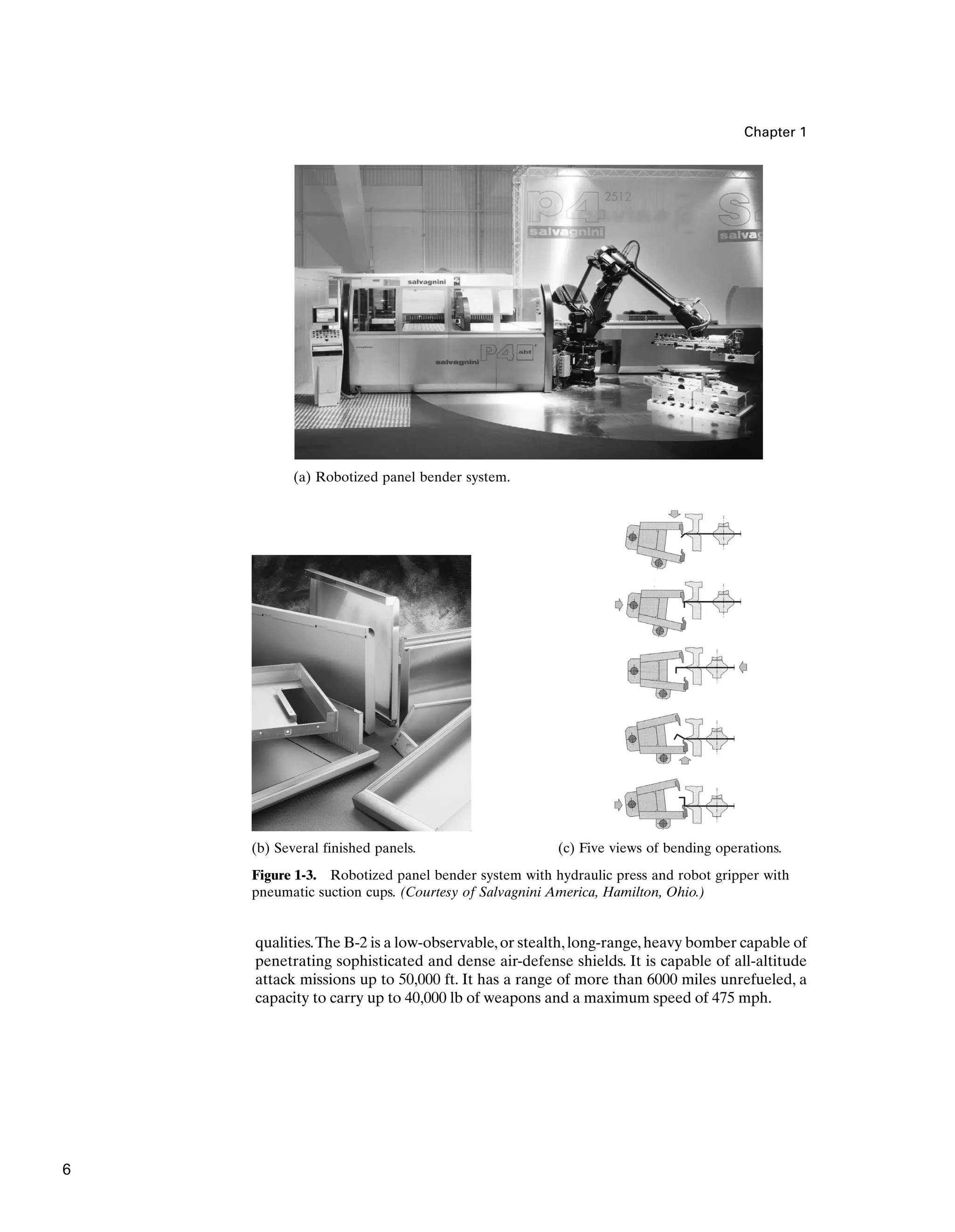
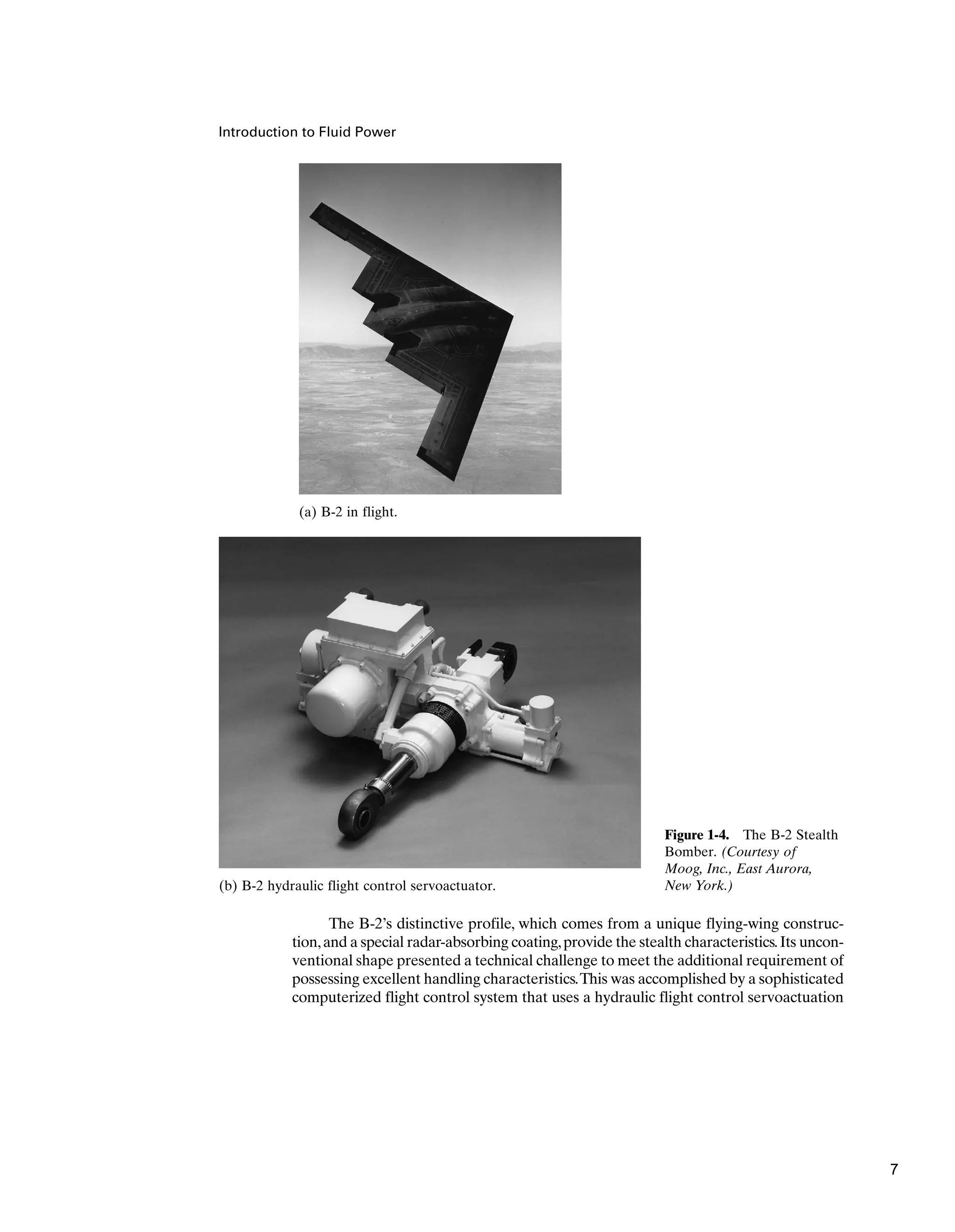
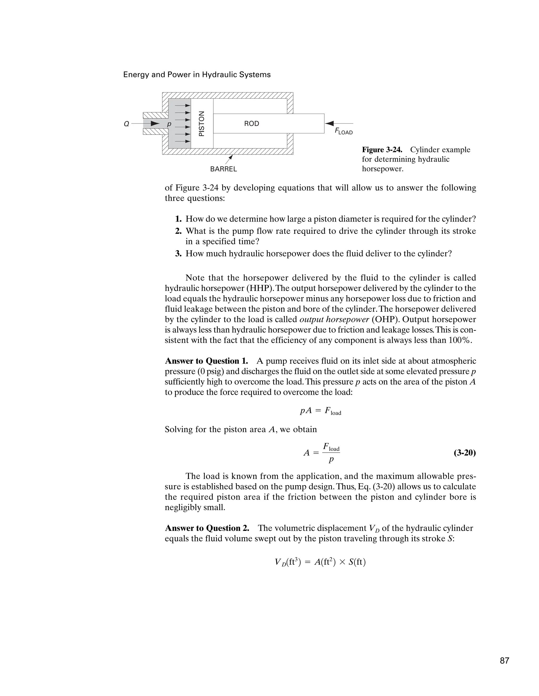
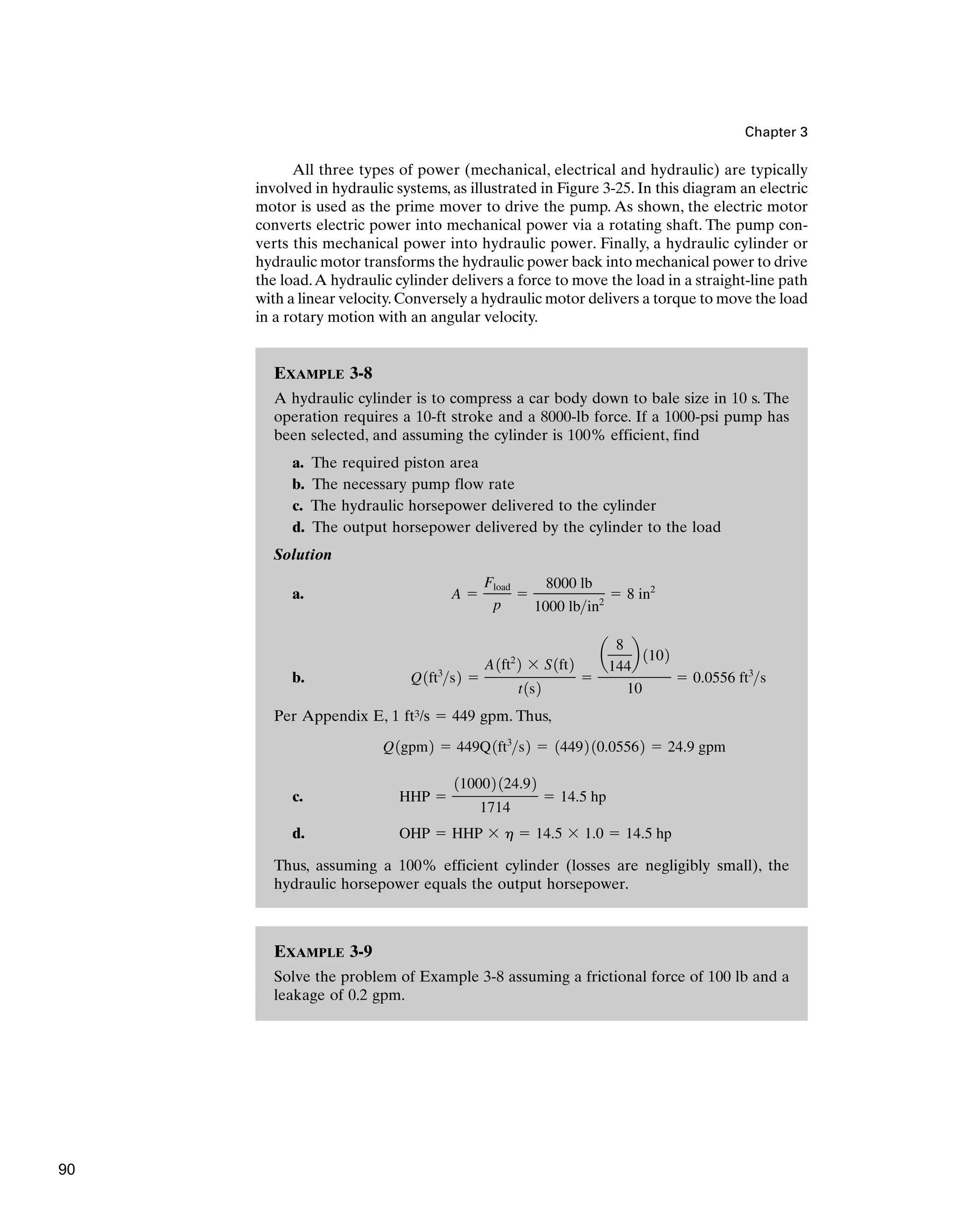
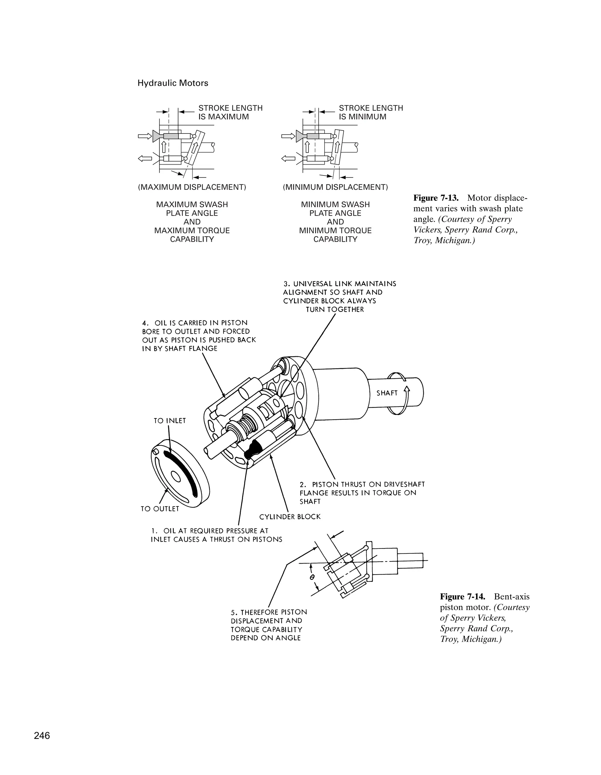
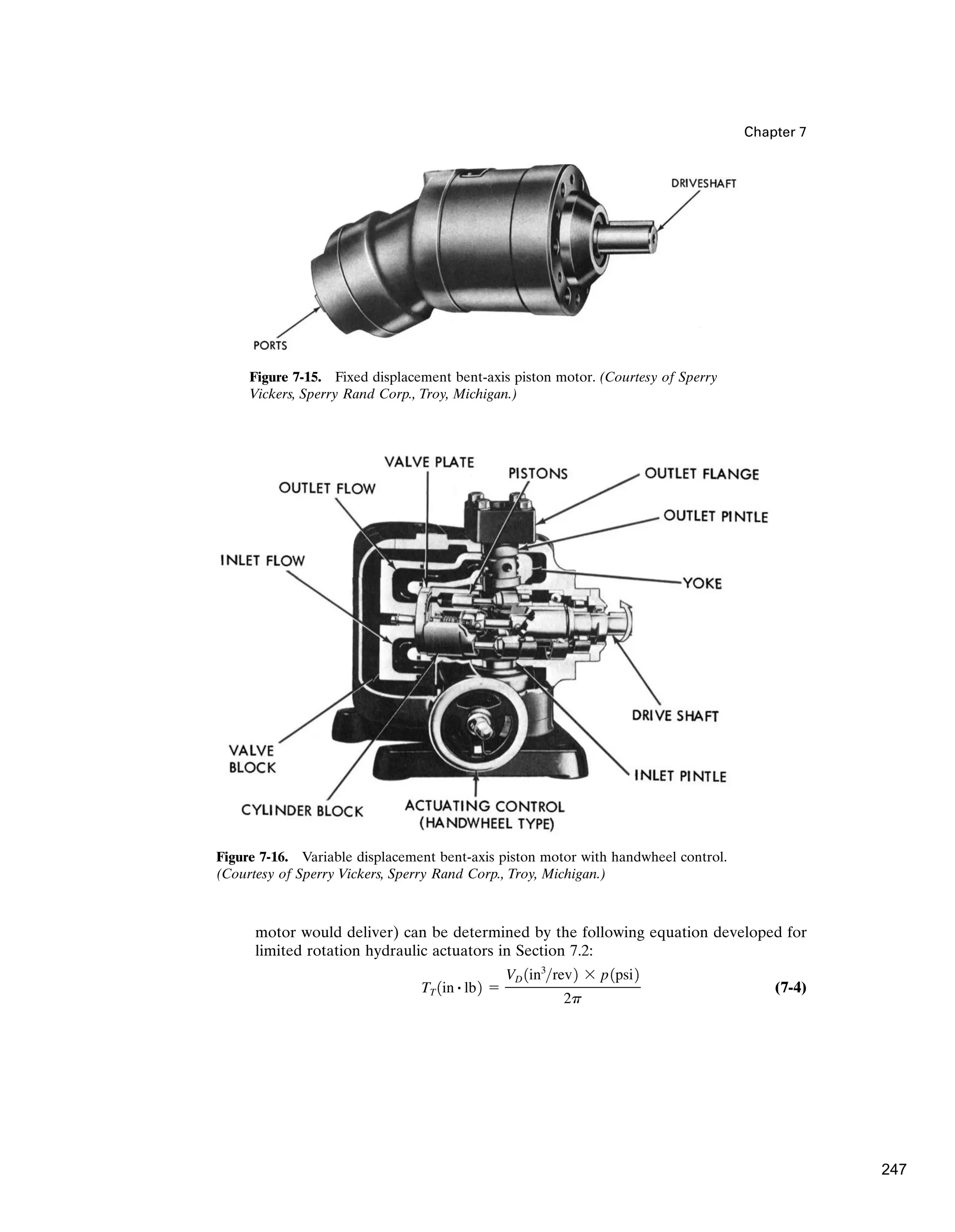
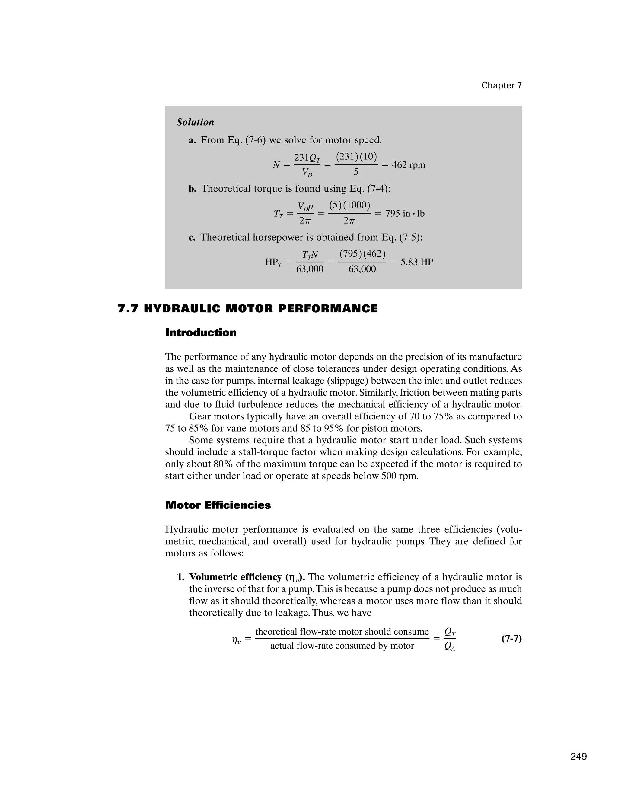
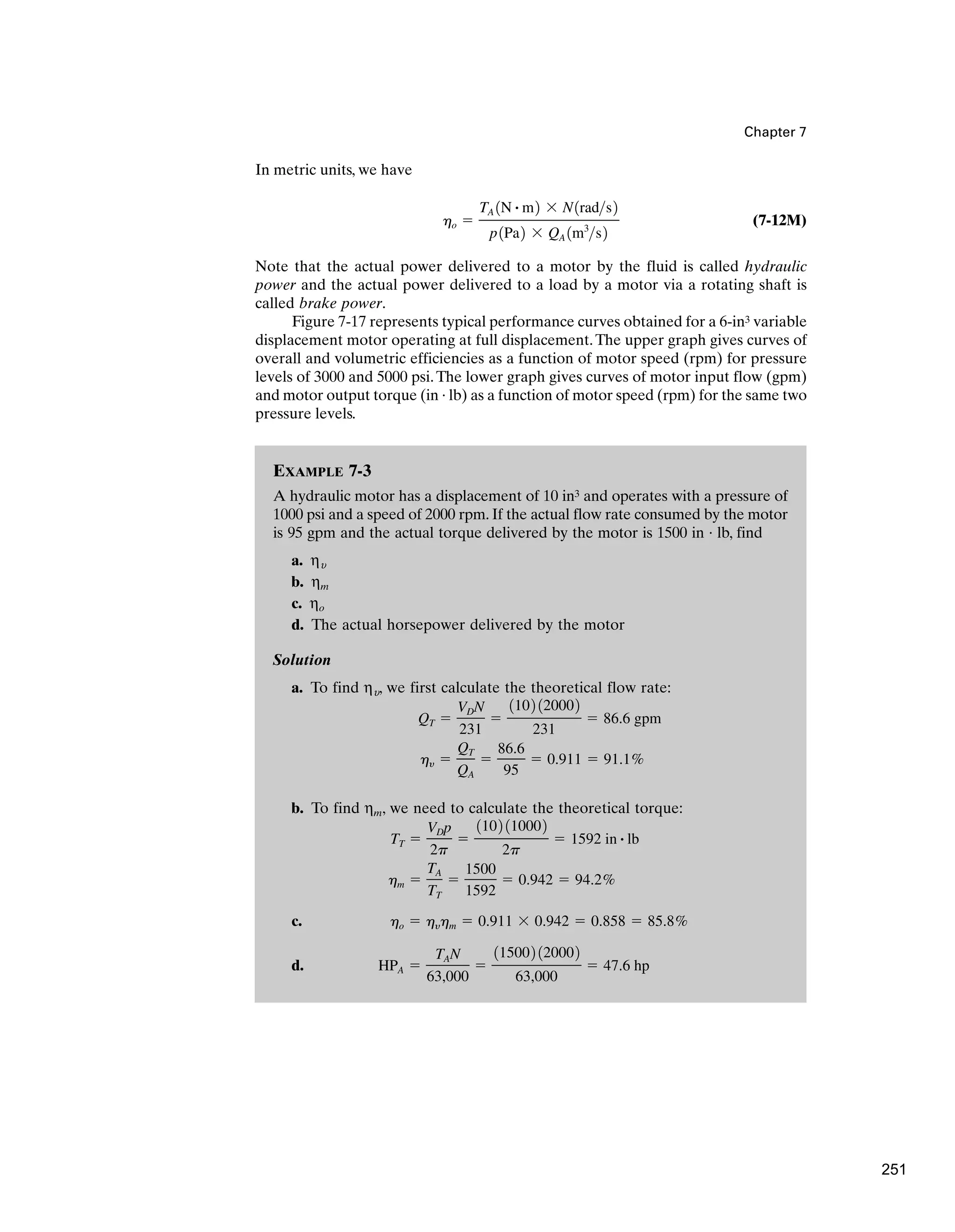
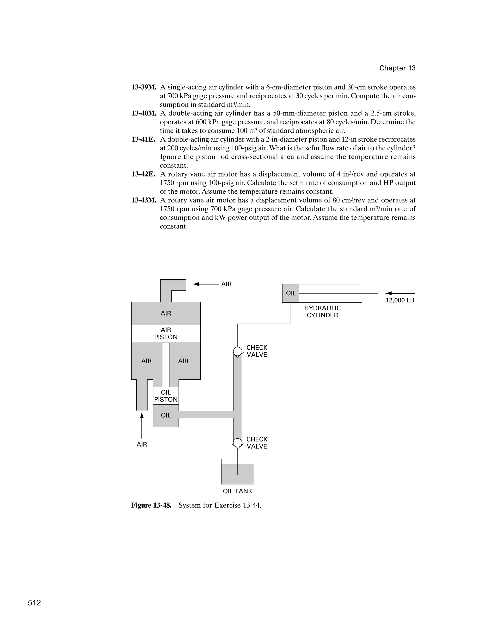
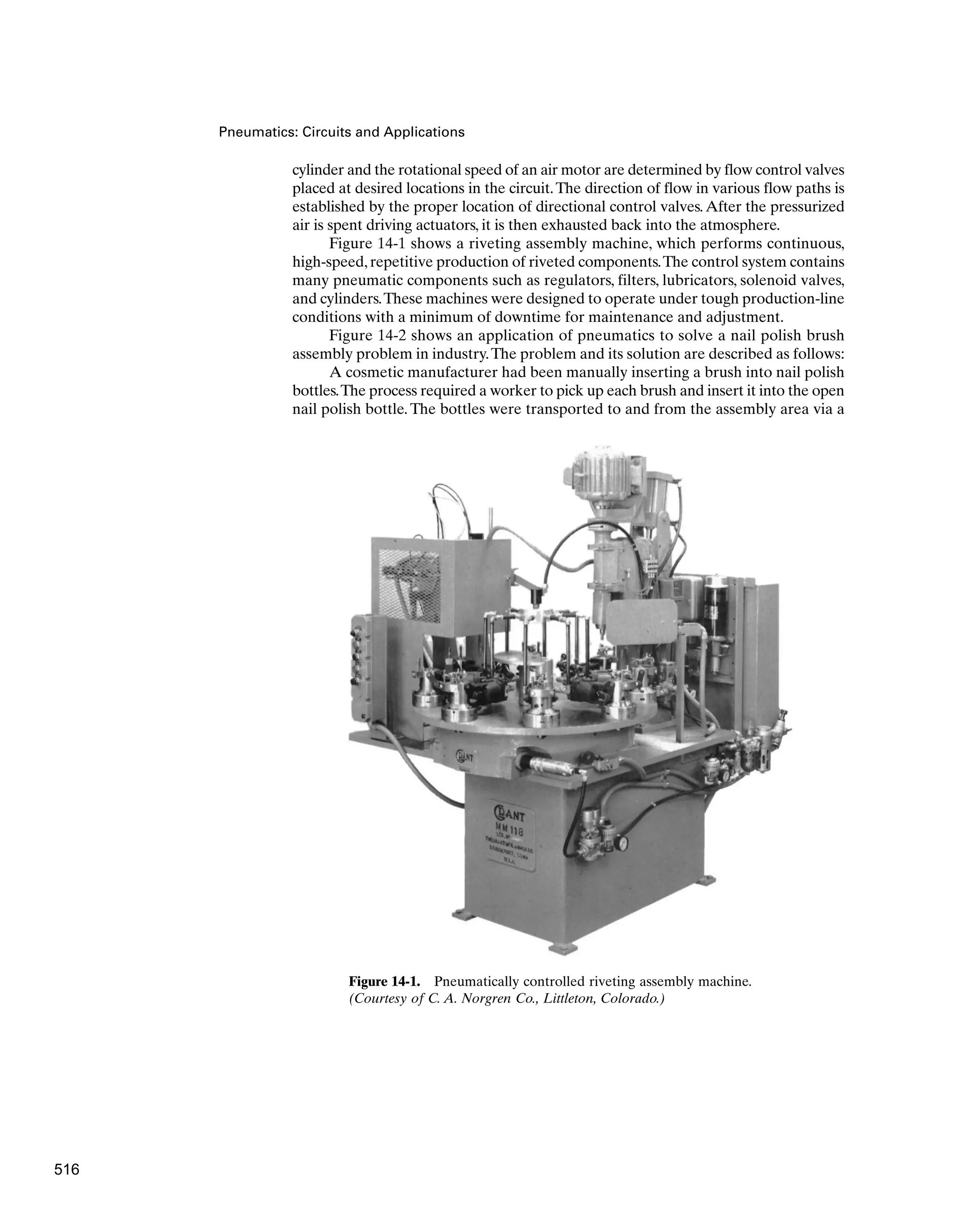
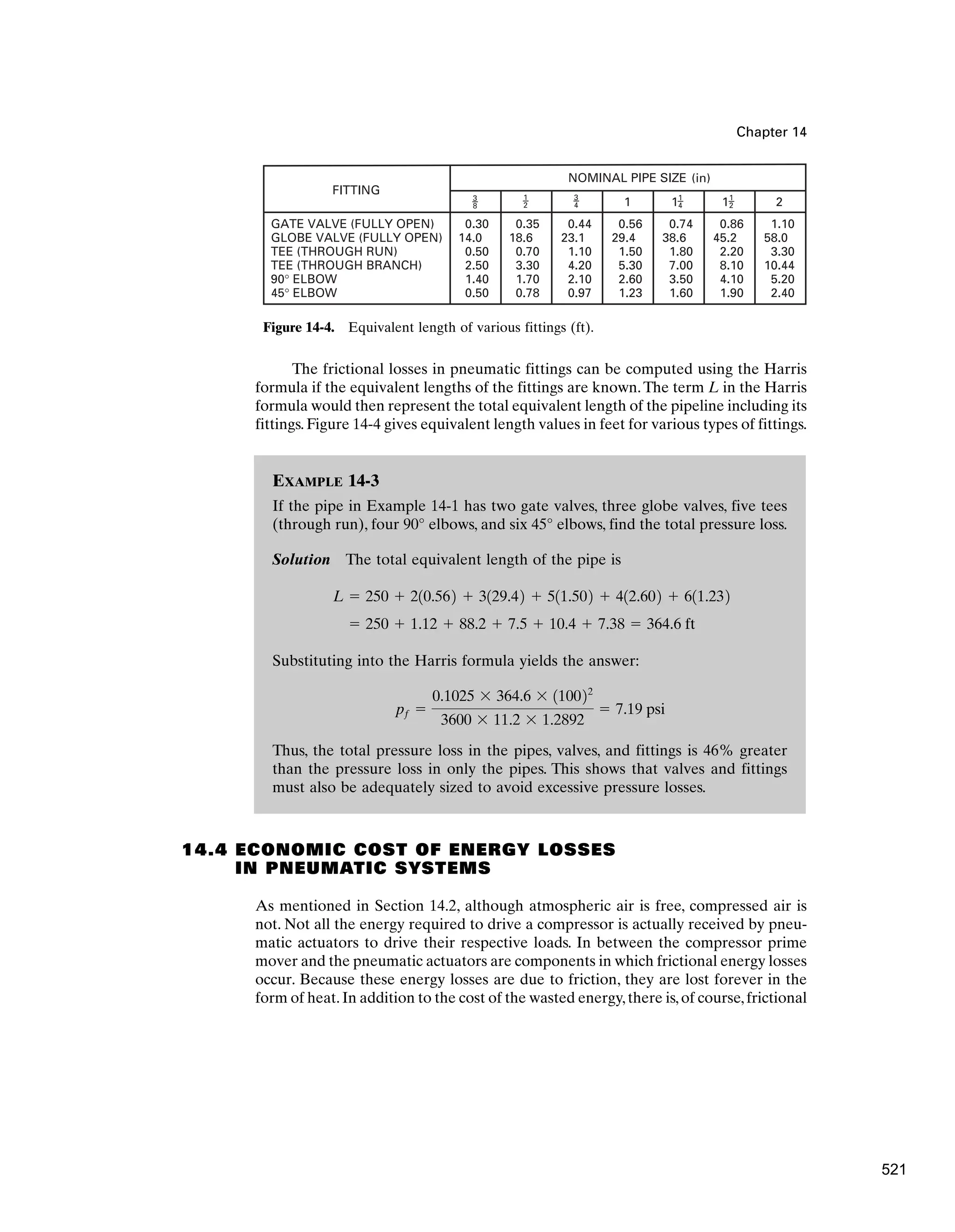
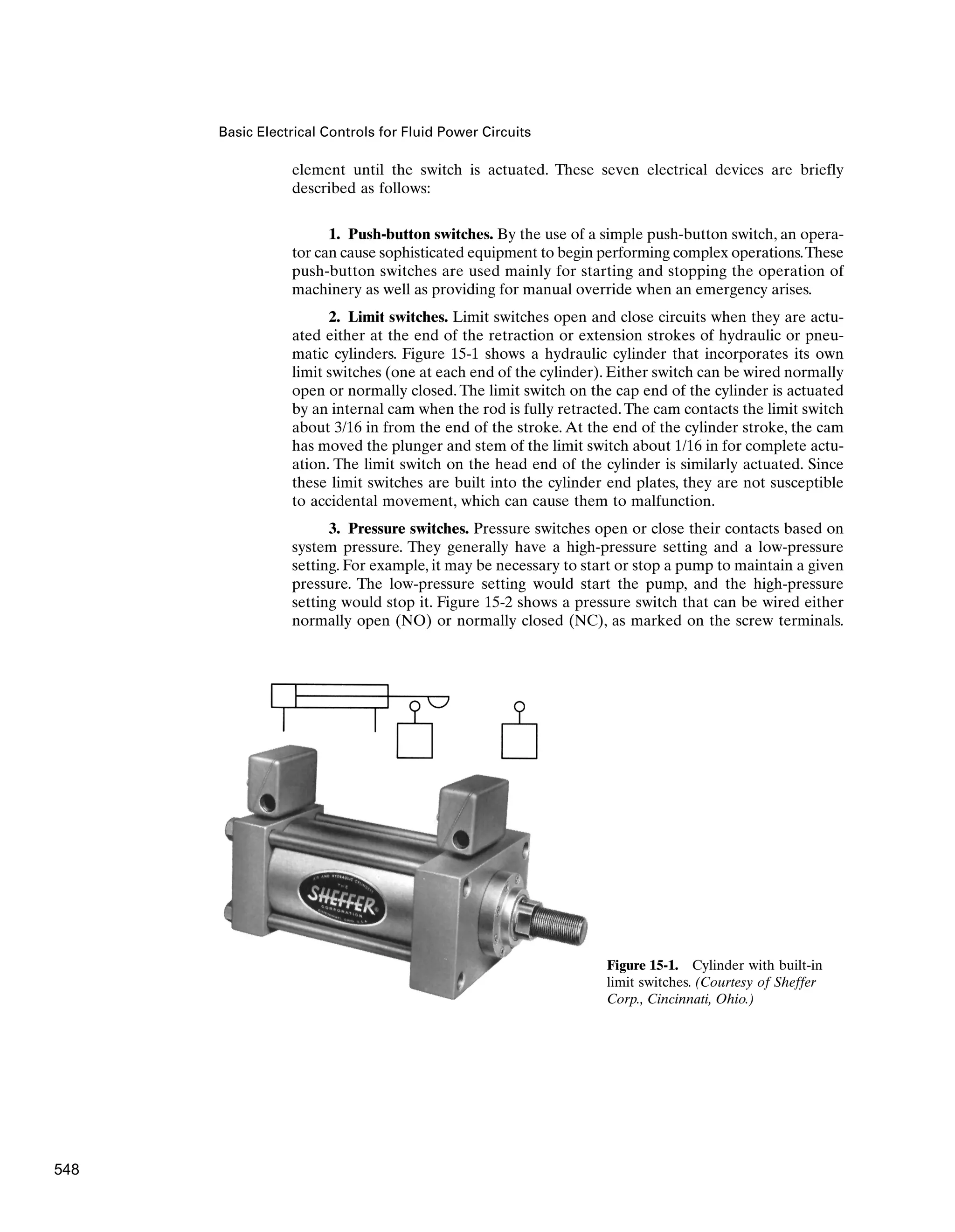
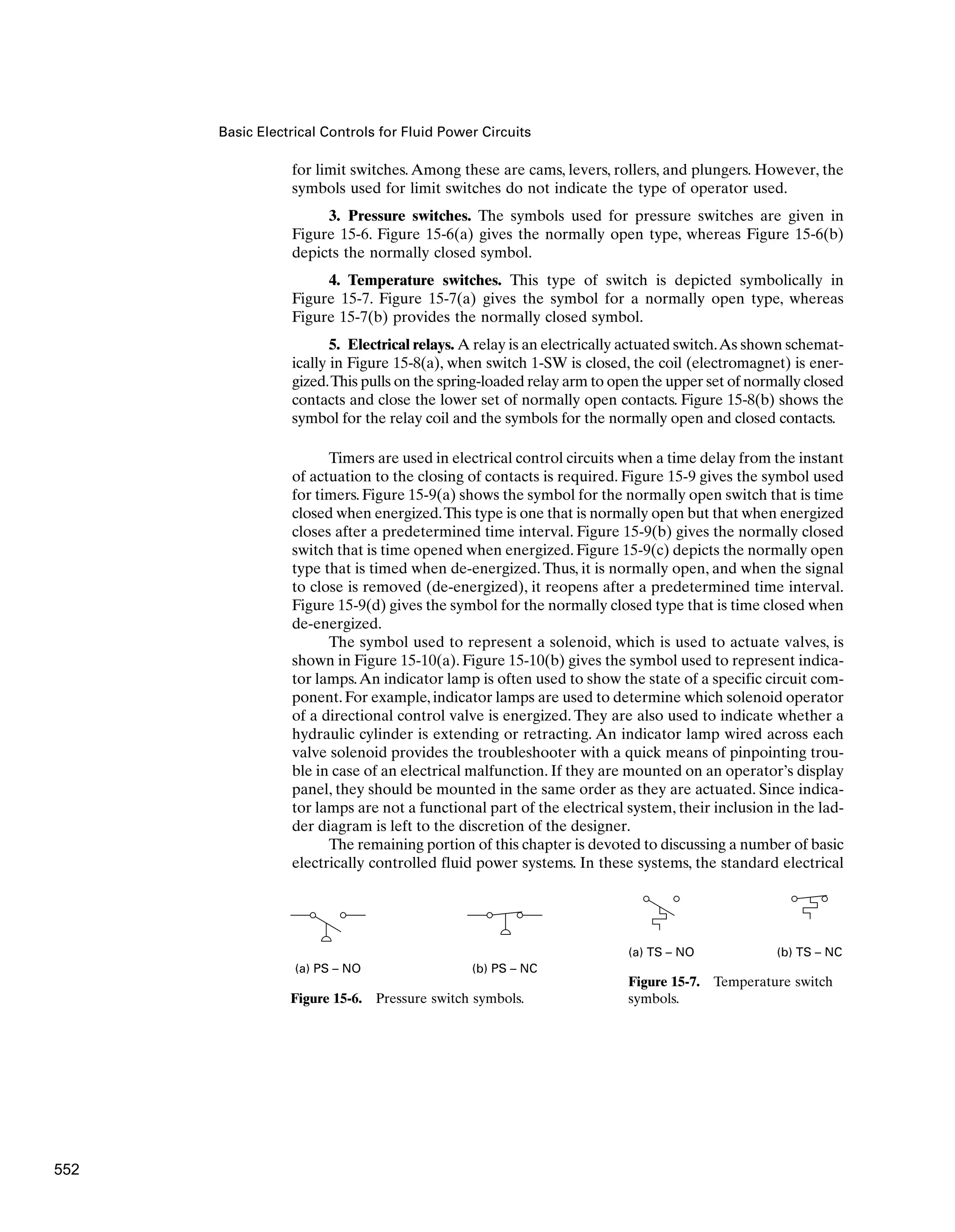
The document is the seventh edition of 'Fluid Power with Applications' by Anthony Esposito, which covers the definition, history, and applications of fluid power technology that utilizes pressurized fluids for generation, control, and transmission of power in various industries. It discusses both hydraulic and pneumatic systems, their components, and their advantages, while highlighting significant historical developments that have shaped the fluid power industry. The content further includes chapters on hydraulic pumps, motors, valves, circuit design, and maintenance, among other topics, reinforcing the critical role fluid power plays in modern manufacturing and machinery.


![Physical Properties of Hydraulic Fluids
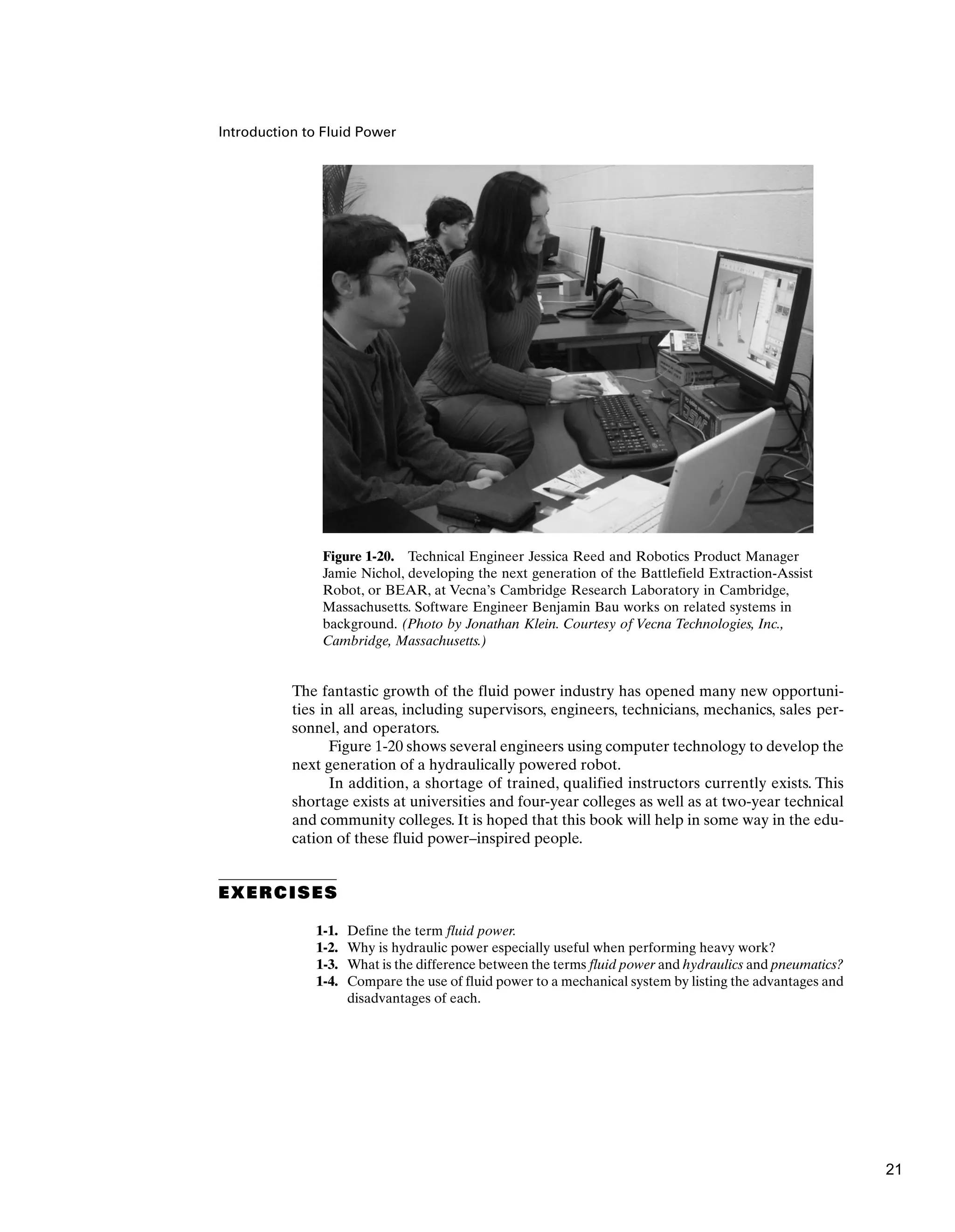
Figure 2-1. Hydraulic fluid
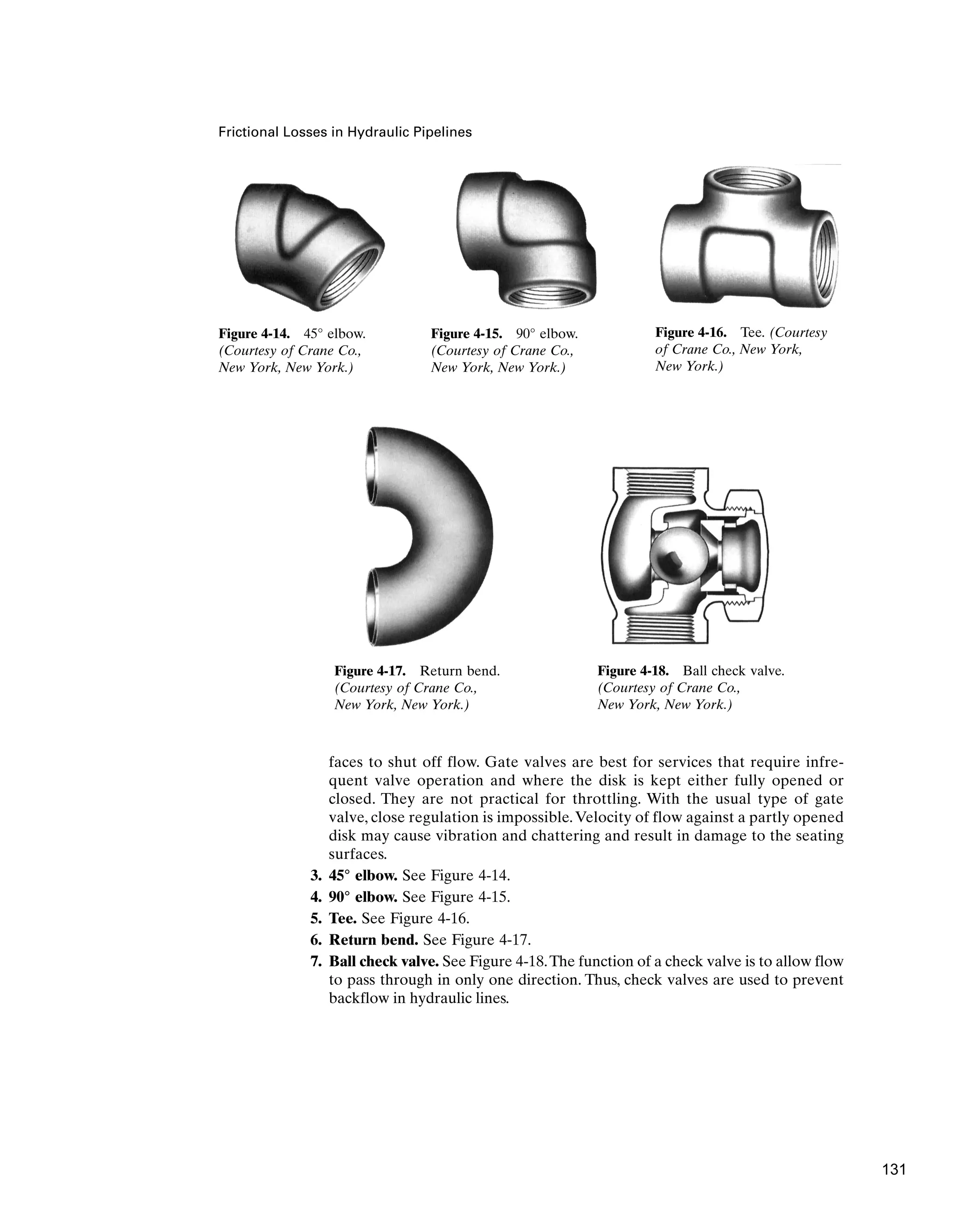
test kit. (Courtesy of Gulf Oil
Corp., Houston, Texas.)
hydraulic systems and the chemical-related properties dealing with maintenance of
the quality of these hydraulic fluids. These properties include rate of oxidation, fire
resistance, foam resistance, lubricating ability, and acidity.
2.2 FLUIDS: LIQUIDS AND GASES
Liquids
The term fluid refers to both gases and liquids. A liquid is a fluid that, for a given
mass,will have a definite volume independent of the shape of its container.This means
that even though a liquid will assume the shape of the container, it will fill only that
part of the container whose volume equals the volume of the quantity of the liquid.
For example, if water is poured into a vessel and the volume of water is not sufficient
to fill the vessel, a free surface will be formed, as shown in Figure 2-2(a). A free
surface is also formed in the case of a body of water, such as a lake, exposed to the
atmosphere [see Figure 2-2(b)].
Liquids are considered to be incompressible so that their volume does not
change with pressure changes.This is not exactly true, but the change in volume due
to pressure changes is so small that it is ignored for most engineering applications.
Variations from this assumption of incompressibility are discussed in Section 2.6,
where the parameter bulk modulus is defined.
Gases
Gases, on the other hand, are fluids that are readily compressible. In addition, their
volume will vary to fill the vessel containing them. This is illustrated in Figure 2-3,
25](https://image.slidesharecdn.com/anthony-esposito-fps-240124091931-2beb0805/75/Fluid-power-system-Anthony-Esposito-FPS-pdf-30-2048.jpg)


![Chapter 8
Figure 8-29. Schematic of sequence valve. (Courtesy of Abex Corp., Denison
Division, Columbus, Ohio.)
graphic symbol for a sequence valve. The pilot line can come from anywhere in the
circuit and not just from directly upstream, as shown.
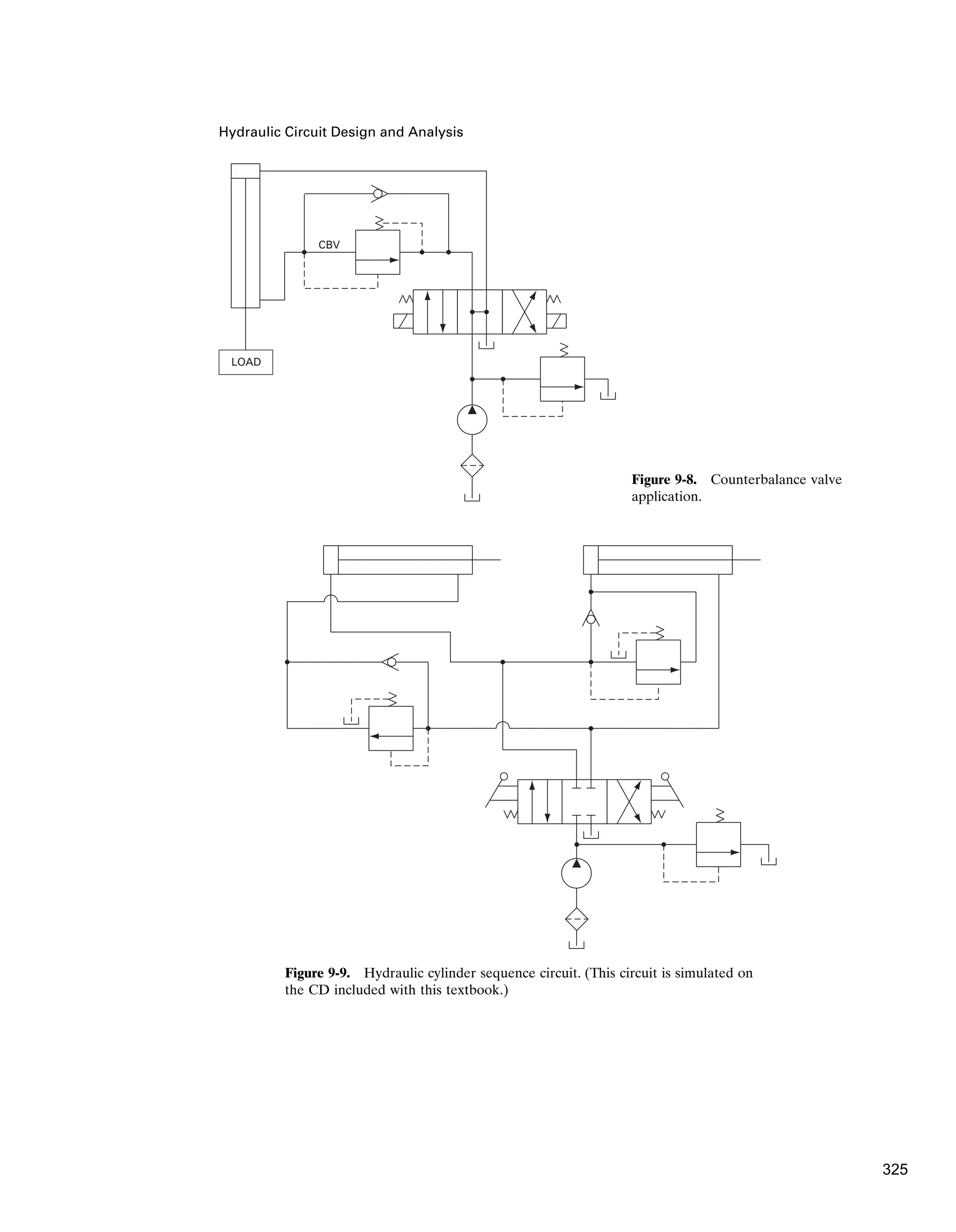
Counterbalance Valves
A final pressure control valve to be presented here is the counterbalance valve (CBV).
The purpose of a counterbalance valve is to maintain control of a vertical hydraulic
cylinder to prevent it from descending due to the weight of its external load.As shown
in Figure 8-30, the primary port of this valve is connected to the bottom of the cylin-
der, and the secondary port is connected to a directional control valve (DCV). The
pressure setting of the counterbalance valve is somewhat higher than is necessary to
prevent the cylinder load from falling due to its weight. As shown in Figure 8-30(a),
when pump flow is directed (via the DCV) to the top of the cylinder, the cylinder
piston is pushed downward. This causes pressure at the primary port to increase to a
value above the pressure setting of the counterbalance valve and thus raise the spool
of the CBV. This then opens a flow path through the counterbalance valve for dis-
charge through the secondary port to the DCV and back to the tank.
When raising the cylinder [see Figure 8-30(b)], an integral check valve opens to
allow free flow for retracting the cylinder. Figure 8-30(c) gives the graphic symbol
for a counterbalance valve. Section 9.7 provides a complete circuit diagram for a
counterbalance valve application.
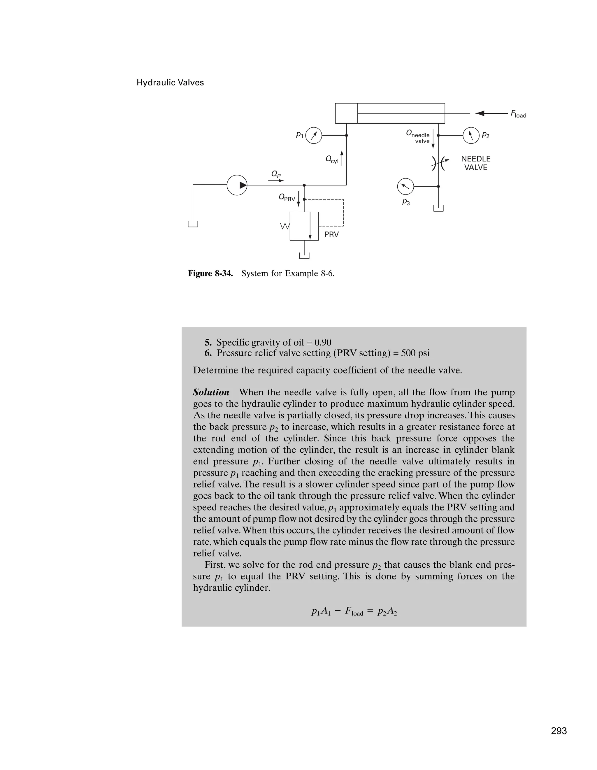
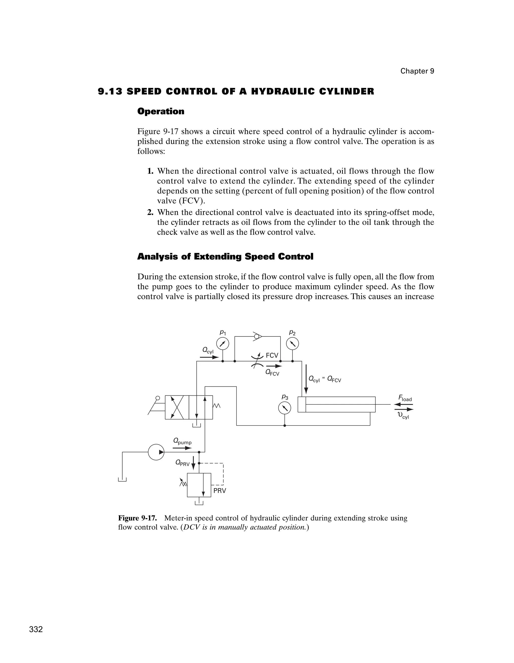
8.4 FLOW CONTROL VALVES
Orifice as a Flow Meter or Flow Control Device
Figure 8-31 shows an orifice (a disk with a hole through which fluid flows) installed
in a pipe. Such a device can be used as a flowmeter by measuring the pressure drop
288](https://image.slidesharecdn.com/anthony-esposito-fps-240124091931-2beb0805/75/Fluid-power-system-Anthony-Esposito-FPS-pdf-293-2048.jpg)


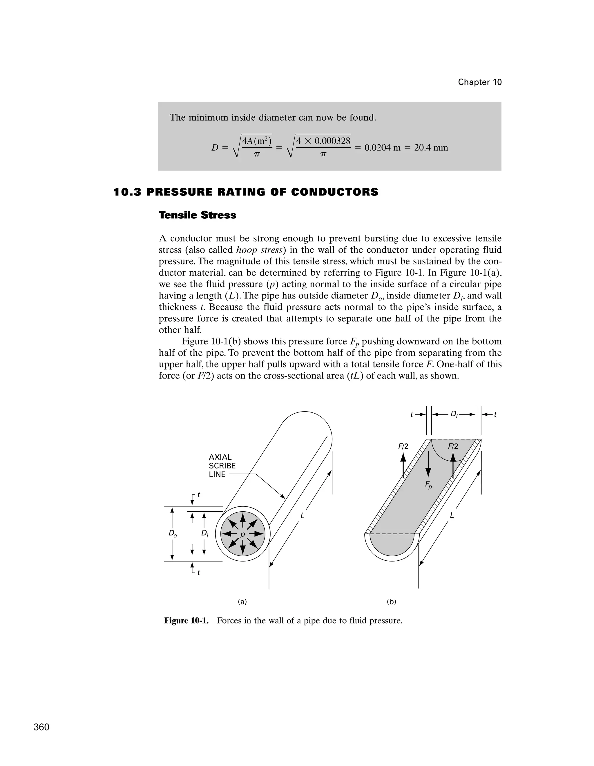


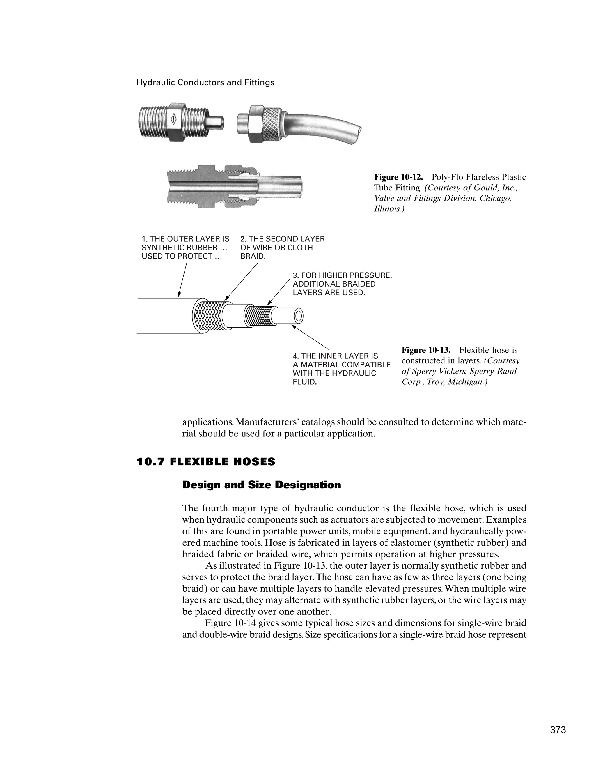
![Hydraulic Conductors and Fittings
TUBE
OD
(in)
1/8
3/16
1/4
5/16
3/8
WALL
THICKNESS
(in)
0.035
0.035
0.035
0.049
0.065
0.035
0.049
0.065
0.035
0.049
0.065
TUBE
ID
(in)
0.055
0.118
0.180
0.152
0.120
0.243
0.215
0.183
0.305
0.277
0.245
TUBE
OD
(in)
1/2
5/8
3/4
WALL
THICKNESS
(in)
0.035
0.049
0.065
0.095
0.035
0.049
0.065
0.095
0.049
0.065
0.109
TUBE
ID
(in)
0.430
0.402
0.370
0.310
0.555
0.527
0.495
0.435
0.652
0.620
0.532
TUBE
OD
(in)
7/8
1
1-1/4
1-1/2
WALL
THICKNESS
(in)
0.049
0.065
0.109
0.049
0.065
0.120
0.065
0.095
0.120
0.065
0.095
TUBE
ID
(in)
0.777
0.745
0.657
0.902
0.870
0.760
1.120
1.060
1.010
1.370
1.310
Figure 10-7. Common tube sizes.
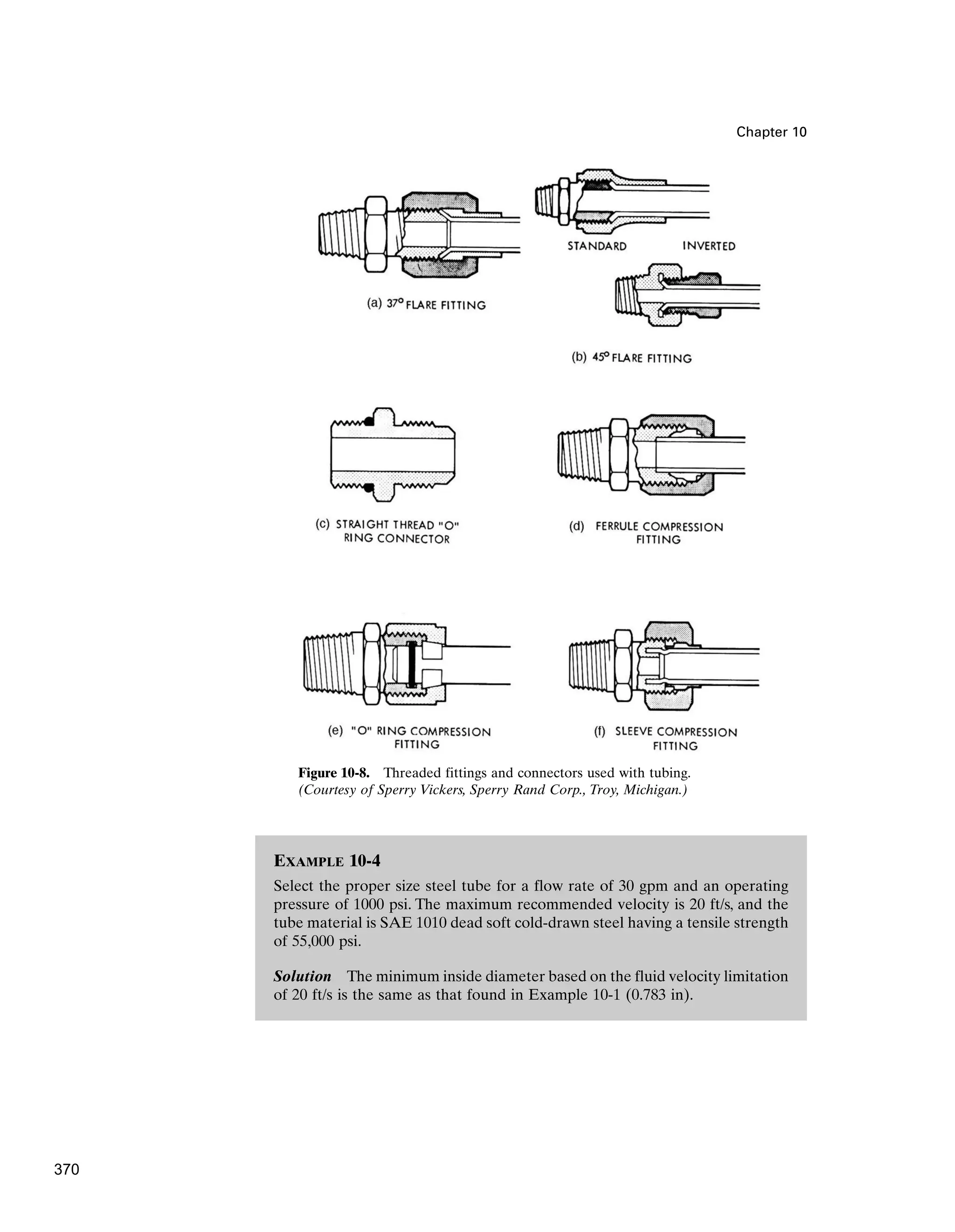
threads on the compression nut. When the hydraulic component has straight thread
ports, straight thread O-ring fittings can be used, as shown in Figure 10-8(c).This type
is ideal for high pressures since the seal gets tighter as pressure increases.
Two assembly precautions when using flared fittings are:
1. The compression nut needs to be placed on the tubing before flaring the tube.
2. These fittings should not be overtightened.Too great a torque damages the seal-
ing surface and thus may cause leaks.
For tubing that can’t be flared, or if flaring is to be avoided, ferrule, O-ring, or
sleeve compression fittings can be used [see Figure 10-8(d), (e), (f)]. The O-ring fit-
ting permits considerable variations in the length and squareness of the tube cut.
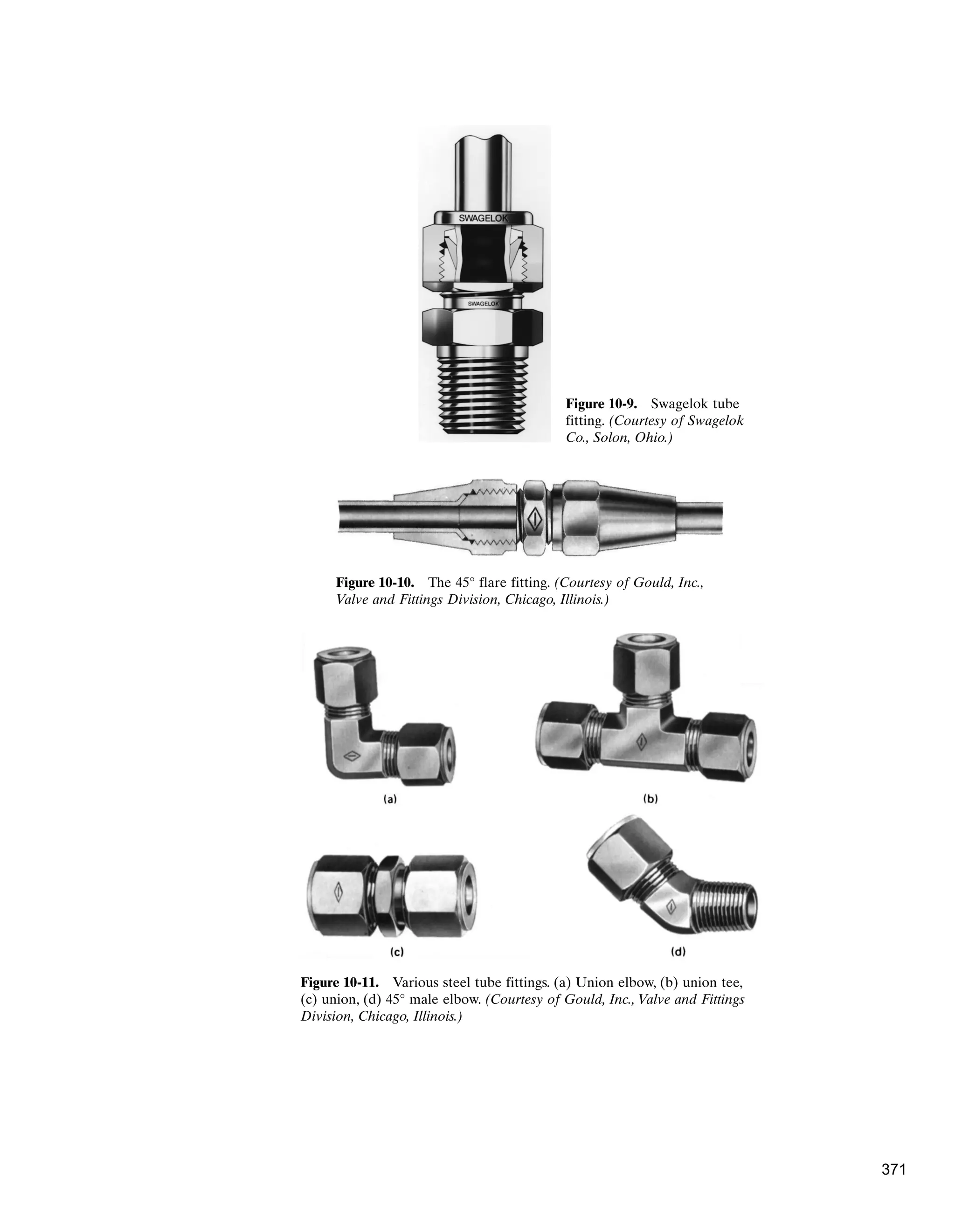
Figure 10-9 shows a Swagelok tube fitting, which can contain any pressure up to
the bursting strength of the tubing without leakage.This type of fitting can be repeat-
edly taken apart and reassembled and remain perfectly sealed against leakage.Assem-
bly and disassembly can be done easily and quickly using standard tools. In the
illustration, note that the tubing is supported ahead of the ferrules by the fitting body.
Two ferrules grasp tightly around the tube with no damage to the tube wall.There is vir-
tually no constriction of the inner wall,ensuring minimum flow restriction.Exhaustive
tests have proven that the tubing will yield before a Swagelok tube fitting will leak.
The secret of the Swagelok fitting is that all the action in the fitting moves along the tube
axially instead of with a rotary motion. Since no torque is transmitted from the fitting
to the tubing,there is no initial strain that might weaken the tubing.The double ferrule
interaction overcomes variation in tube materials, wall thickness, and hardness.
In Figure 10-10 we see the 45° flare fitting.The flared-type fitting was developed
before the compression type and for some time was the only type that could suc-
cessfully seal against high pressures.
Four additional types of tube fittings are depicted in Figure 10-11: (a) union
elbow, (b) union tee, (c) union, and (d) 45° male elbow.With fittings such as these, it
is easy to install steel tubing as well as remove it for maintenance purposes.
369](https://image.slidesharecdn.com/anthony-esposito-fps-240124091931-2beb0805/75/Fluid-power-system-Anthony-Esposito-FPS-pdf-374-2048.jpg)


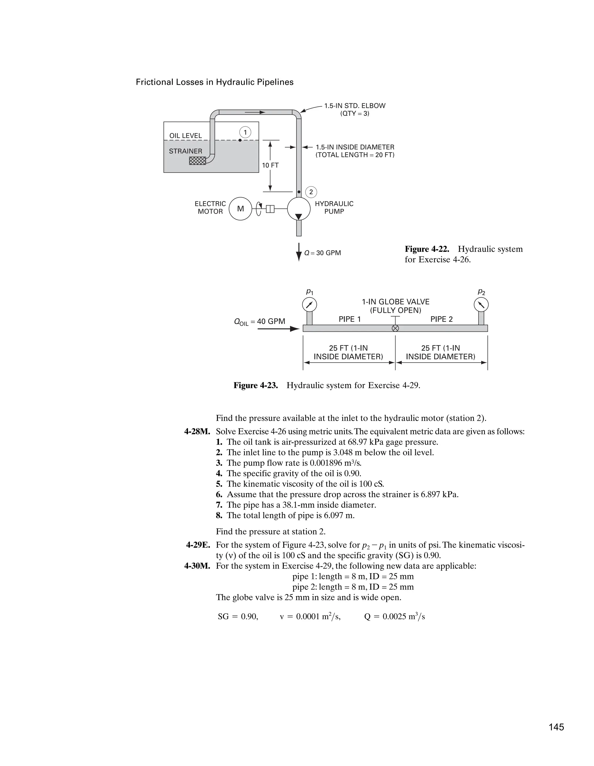
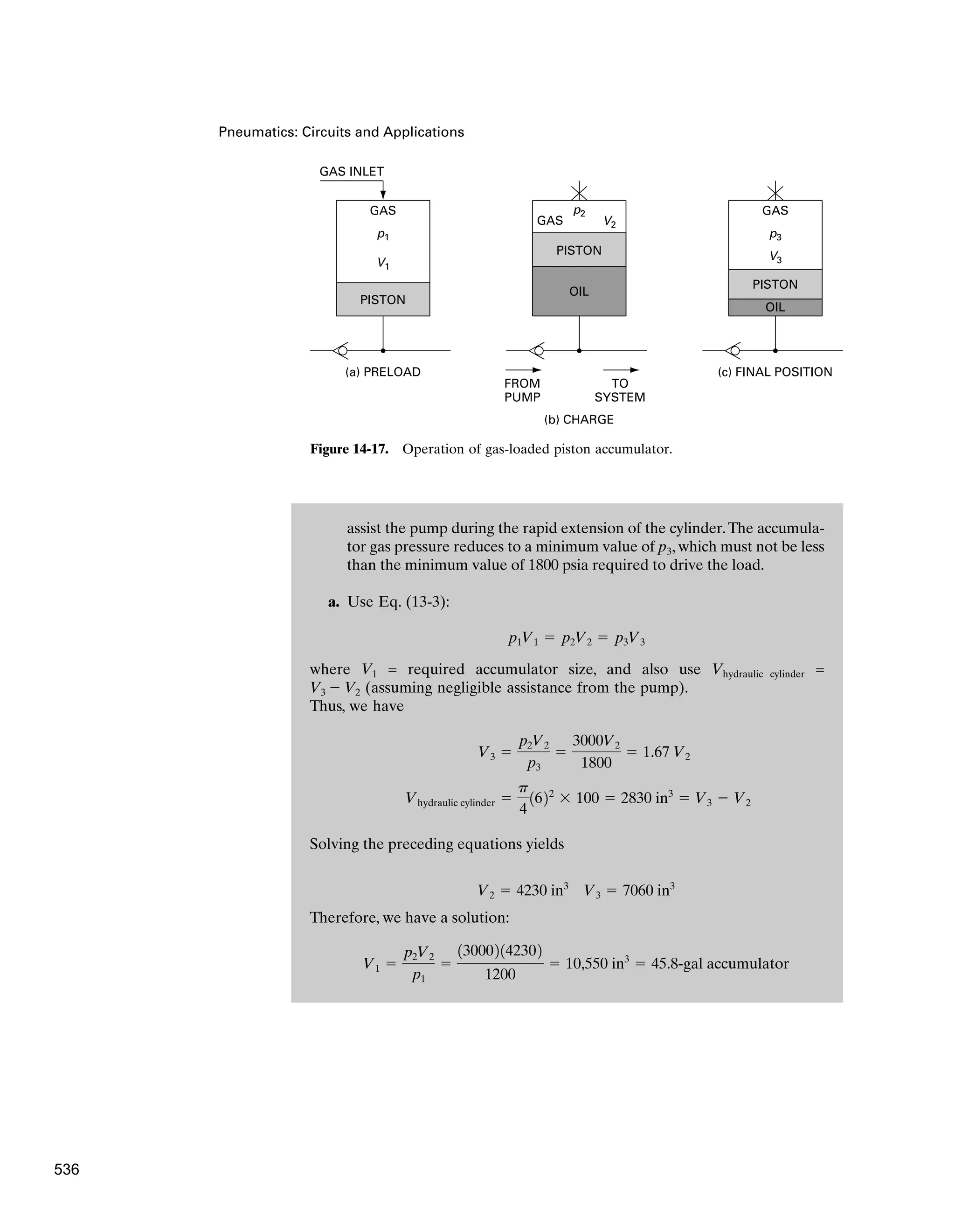
![crushing strokes is 5 min. The following accumulator gas absolute pressures
are given:
a. Calculate the required size of the accumulator.
b. What are the pump hydraulic horsepower and flow requirements with
and without an accumulator?
Solution Figure 14-17 shows the three significant accumulator operating
conditions:
1. Preload [Figure 14-17(a)].This is the condition just after the gas has been
introduced into the top of the accumulator. Note that the piston (assum-
ing a piston design) is all the way down to the bottom of the accumulator.
2. Charge [Figure 14-17(b)].The pump has been turned on, and hydraulic
oil is pumped into the accumulator since p2 is greater than p1. During this
phase, the four-way valve is in its spring-offset position.Thus, system pres-
sure builds up to the 3000-psia level of the pressure relief valve setting.
3. Final position of accumulator piston at end of cylinder stroke [Figure
14-17(c)].The four-way valve is actuated to extend the cylinder against its
load. When the system pressure drops below 3000 psia, the accumulator
3000-psia gas pressure forces oil out of the accumulator into the system to
p3 ⫽ minimum pressure required to actuate load ⫽ 1800 psia
⫽ 3000 psia ⫽ pressure relief valve setting
p2 ⫽ gas charge pressure when pump is turned on
p1 ⫽ gas precharge pressure ⫽ 1200 psia
Chapter 14
FLOAD
Figure 14-16. Use of gas-loaded
accumulator in hydraulic system
for crushing car bodies.
535](https://image.slidesharecdn.com/anthony-esposito-fps-240124091931-2beb0805/75/Fluid-power-system-Anthony-Esposito-FPS-pdf-540-2048.jpg)


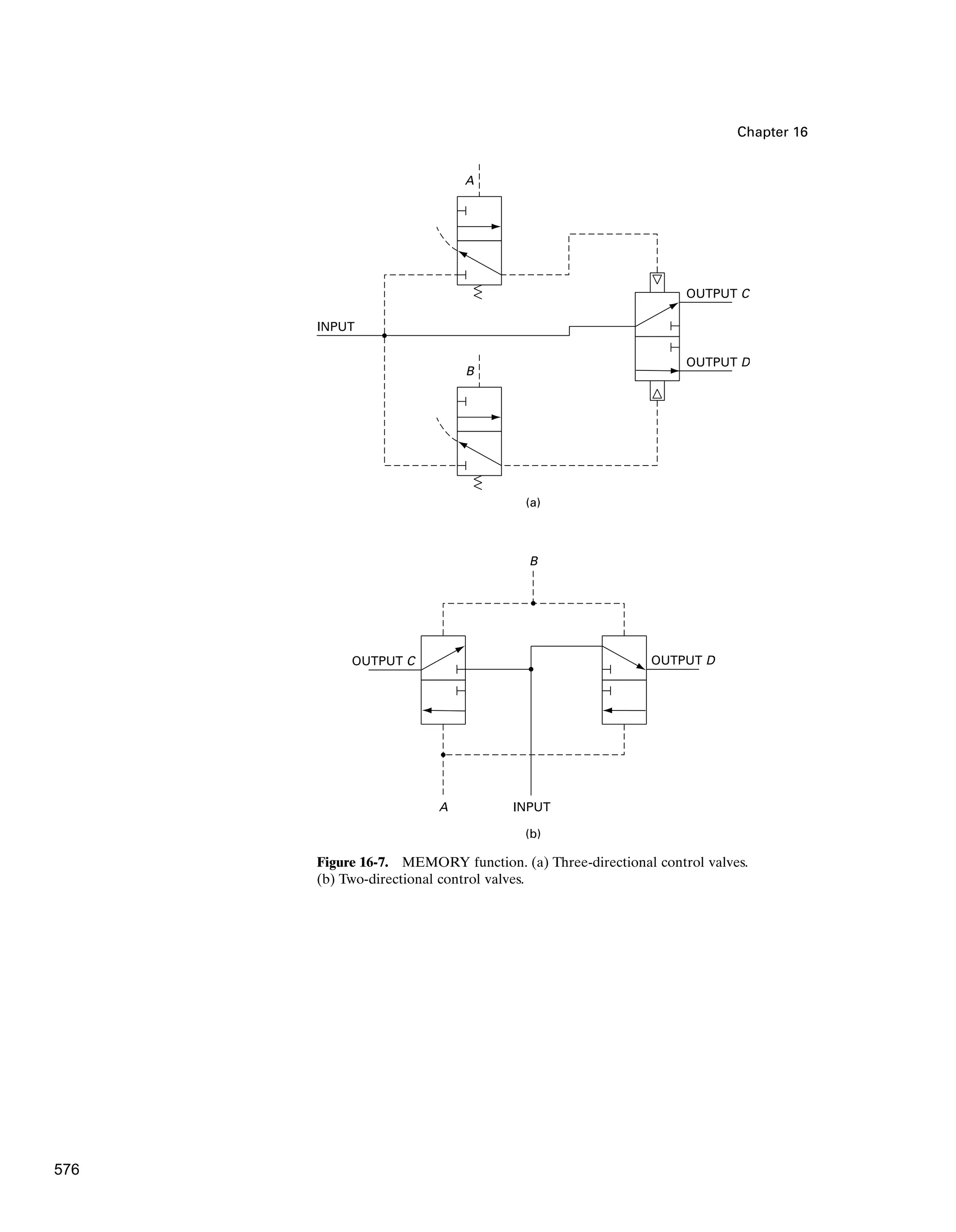
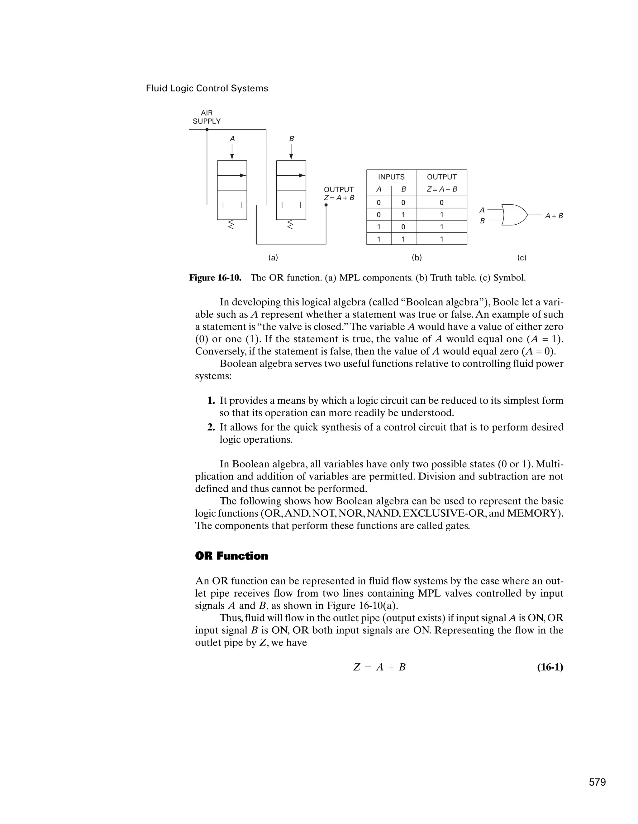
![Fluid Logic Control Systems
2. It allows for a quick synthesis of a control circuit that is to perform desired logic
operations.
These two useful functions can be accomplished for both MPL control systems
and electrical control systems.
16.2 MOVING-PART LOGIC (MPL) CONTROL SYSTEMS
Introduction
Moving-part logic (MPL) control systems use miniature valve-type devices, each
small enough to fit in a person’s hand. Thus, an entire MPL control system can be
placed in a relatively small space due to miniaturization of the logic components.
Figure 16-2 shows a miniature three-way limit valve along with its outline dimen-
sions of in long by in by in. This valve, which is designed to give depend-
able performance in a small, rugged package, has a stainless steel stem extending
in from the top. The valve design is a poppet type with fast opening and high
flow 7.0 CFM at 100-psi air (working range is 0 to 150 psi). Mounted on a machine
or fixture, the valve is actuated by any moving part that contacts and depresses
the stem.
Figure 16-3(a) shows an MPL circuit manifold, which is a self-contained mod-
ular subplate with all interconnections needed to provide a “two-hand-no-tie-down”
pneumatic circuit. The manifold is designed to be used with three modular plug-in
control valves and to eliminate the piping time and materials normally associated
with circuitry. The main function of this control system is to require a machine
operator to use both hands to actuate the machinery, thus ensuring that the opera-
tor’s hands are not in a position to be injured by the machine as it is actuated.When
used with two guarded palm button valves [see Figure 16-3(b)], which have been
1
8
1
2
3
4
1 3
16
Figure 16-2. Miniature three-way limit valve. (Courtesy of Clippard Instrument Laboratory,
Inc., Cincinnati, Ohio.)
571](https://image.slidesharecdn.com/anthony-esposito-fps-240124091931-2beb0805/75/Fluid-power-system-Anthony-Esposito-FPS-pdf-576-2048.jpg)


![Advanced Electrical Controls for Fluid Power Systems
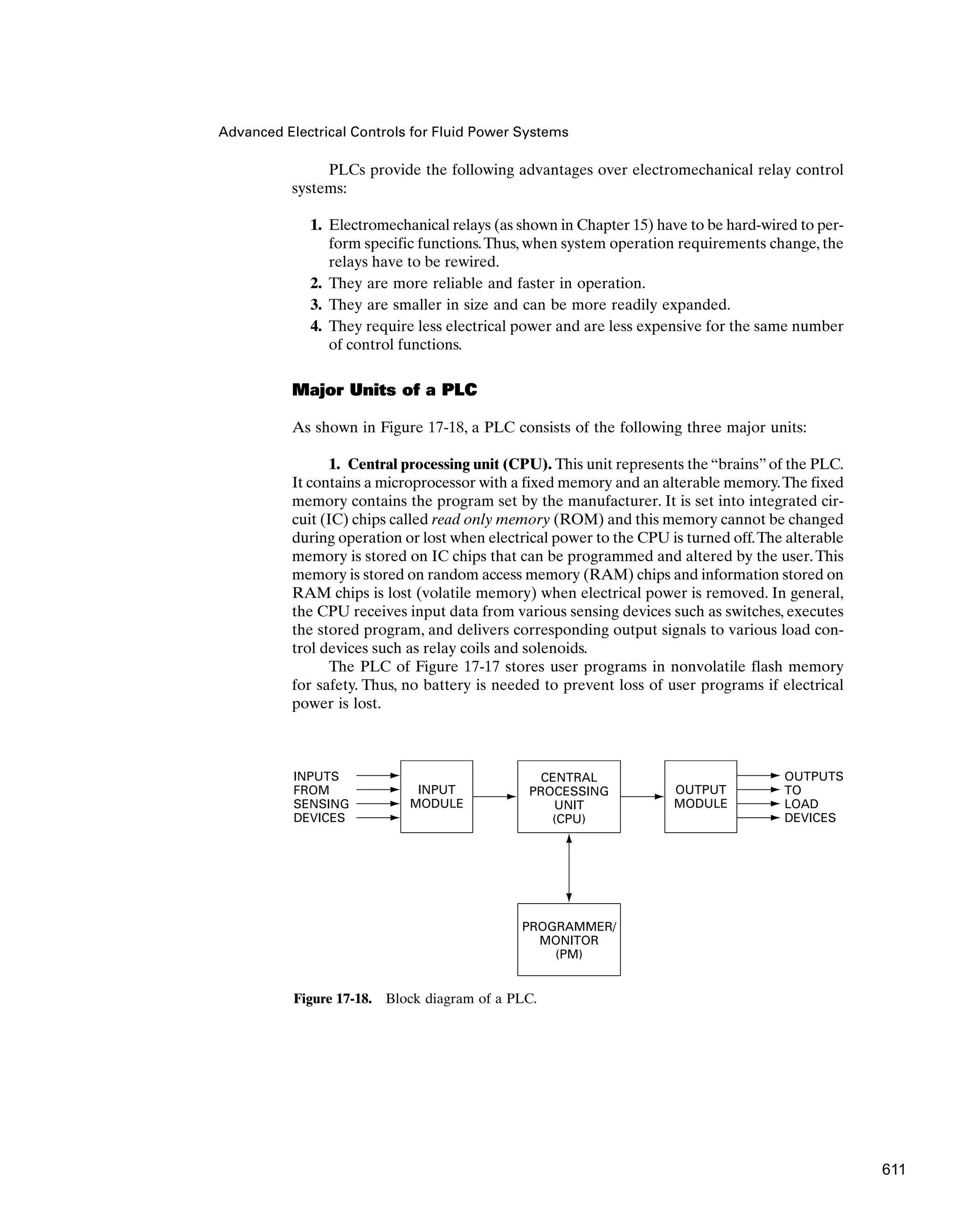
3. Input/output module (I/O). This module is the interface between the fluid
power system input sensing and output load devices and the CPU.The purpose of the
I/O module is to transform the various signals received from or sent to the fluid power
interface devices such as push-button switches,pressure switches,limit switches,motor
relay coils, solenoid coils, and indicator lights.These interface devices are hard-wired
to terminals of the I/O module.
The PLC of Figure 17-17 contains a powerful 16-bit, 20-MHz processor. Multi-
tasking of up to 64 programs allows the user to divide the control task into manage-
able objects. As shown in Figure 17-17, this PLC contains 12 inputs and 8 outputs,
each of which are monitored by light-emitting diodes.This PLC can be programmed
off-line in a ladder logic diagram using a microcomputer. Capabilities include proj-
ect creation, program editing, loading, and documentation. The system allows the
user to monitor the controlled process during operation and provides immediate
information regarding the status of timers, counters, inputs, and outputs.
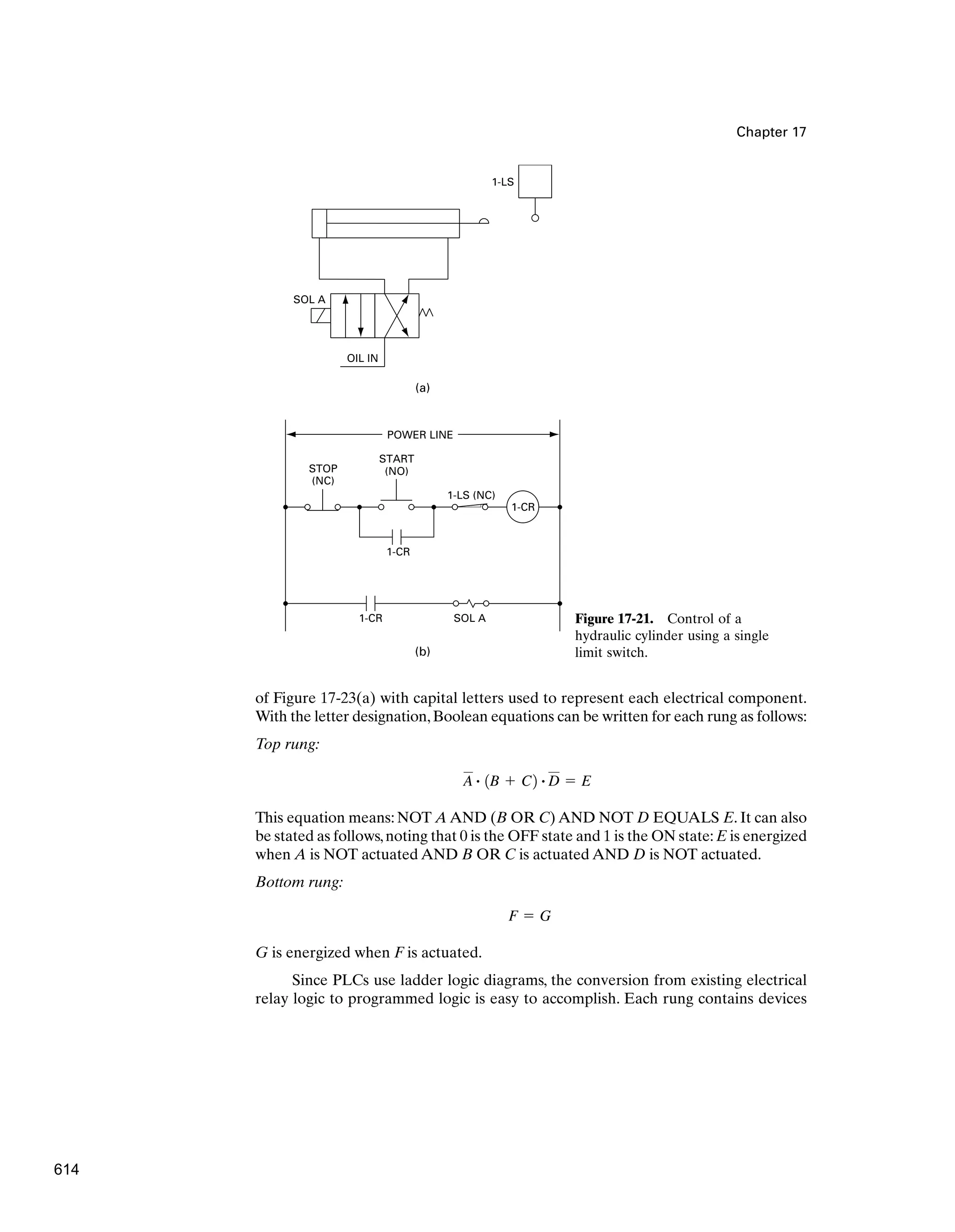
PLC Control of a Hydraulic Cylinder
To show how a PLC operates, let’s look at the system of Figure 15-11 (repeated in
Figure 17-21), which shows the control of a hydraulic cylinder using a single limit
switch.
For this system, the wiring connections for the input and output modules are
shown in Figure 17-22(a) and (b), respectively. Note that there are three sensing
input devices to be connected to the input module and one output control/load
device to be connected to the output module. The electrical relay is not included
in the I/O connection diagram since its function is replaced by an internal PLC
control relay.
The PLC ladder logic diagram that would be constructed and programmed into
the memory of the CPU is shown in Figure 17-23(a). Note that the layout of the PLC
ladder diagram [Figure 17-23(a)] is similar to the layout of the hard-wired relay lad-
der diagram (Figure 17-21).The two rungs of the relay ladder diagram are converted
to two rungs of the PLC ladder logic diagram.The terminal numbers used on the I/O
connection diagram are the same numbers used to identify the electrical devices on
the PLC ladder logic diagram.The symbol — — represents a normally closed set of
contacts and the symbol —||— represents a normally open set of contacts.The sym-
bol —( )— with number 030 represents the relay coil that controls the two sets of
contacts with number 030, which is the address in memory for this internal relay.The
relay coil and its two sets of contacts are programmed as internal relay equivalents.
The symbol —( )— with number 010 represents the solenoid.
A PLC is a digital solid-state device and thus performs operations based on the
three fundamental logic functions: AND, OR, and NOT. Each rung of a ladder dia-
gram can be represented by a Boolean equation.The hard-wired ladder diagram logic
is fixed and can be changed only by modifying the way the electrical components are
wired. However, the PLC ladder diagram contains logic functions that are program-
mable and thus easily changed. Figure 17-23(b) shows the PLC ladder logic diagram
||
613](https://image.slidesharecdn.com/anthony-esposito-fps-240124091931-2beb0805/75/Fluid-power-system-Anthony-Esposito-FPS-pdf-618-2048.jpg)