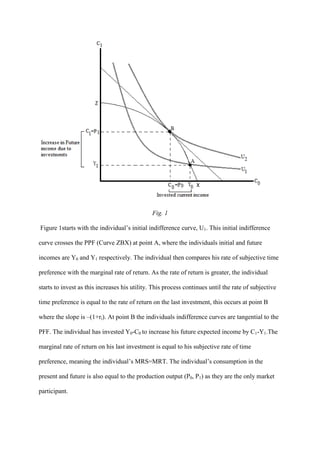
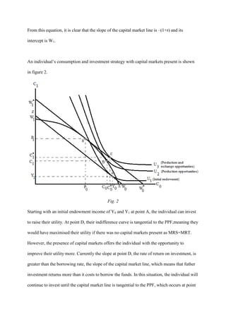
1) A rational economic agent in a two-period economy without capital markets must decide how to allocate their initial endowment income between current and future consumption. They do this by analyzing indifference curves and comparing their subjective rate of time preference to production opportunities. 2) With capital markets, the agent can borrow or lend at the market interest rate. This creates a capital market line that allows higher utility. The agent invests until the marginal rate of return equals the interest rate, then borrows along the capital market line until their time preference equals the interest rate. 3) The maximum the businessman will pay for insurance is £114,941.55 if he has logarithmic utility. His expected wealth is £170,

1. 1). Consider investment/production and consumption of one person in a simple two -
period economy without capital markets. Use diagrams to describe investment and
consumption of this rational individual given a subjective rate of time preference. Extend
your analysis of this rational individual by allowing for capital markets to exist.
Compare and contrast your results with the ones from the previous discussion.
A rational economic agent in a one-person/one-good two-period economy without the
presence of capital marketshas a choice of how he uses his initial endowment income, Yo,
and his end of period income, Y1. He can decide how much of the income to consume now,
Co, and how much he should invest in production to consume in the future, C1.
Theassumptions of this economy are that all actions are undertaken with certainty; for
example, the actions of investment are known. There are also no transaction costs and it is
also assumed that the marginal utility of consumption is positive but decreasing.
For the individual to be able to decide whether to consume now or invest to consume in the
future, he needs to know his subjective trade-offs that must be made between consumption
now and consumption in the future.This is achieved through analysing his utility functions
and indifference curves.
The slope of any point on the indifference curves shows the rate which C0 and C1 can be
traded for each other; this is called the marginal rate of substitution (MRS). The MRS can be
shown algebraically as
This equation introduces the decision maker’s subjective rate of time preference, . The
subjective rate of time preference represents the individual’s optimal rate of exchange
between present and future consumption, it is unique to each person. It shows how much

2. future consumption must be received, to make investment today worthwhile and still keep the
same total utility.
Production opportunities then allow the individual to invest a current unit to be turned into
more than one unit for future consumption. The individual’s schedule of production
opportunities shows the possible combinations of current and future income that the
individual could attain through investment and de-investment. The individual willinvest in all
opportunities which yield a higher rate of return than their own subjective rate of time
preference. The Production Possibilities Frontier (PPF) curve aggregates all possible
investment opportunities schedules. The slope of a line tangent to the PPF is called the
marginal rate of transformation (MRT), which is “the rate at which one dollar of consumption
forgone today is transformed by productive investment into a dollar of consumption
tomorrow.”1
Given an individual’s subjective rate of time preference, , the individual’s current and
future consumption can be derived.
1 rd
Quoted from page 7, Copeland, T.E. and Weston, J.F., 1992.Financial Theory and Corporate Policy 3 ed.
Addison-Wesley.

3. Z
X
Fig. 1
Figure 1starts with the individual’s initial indifference curve, U1. This initial indifference
curve crosses the PPF (Curve ZBX) at point A, where the individuals initial and future
incomes are Y0 and Y1 respectively. The individual then compares his rate of subjective time
preference with the marginal rate of return. As the rate of return is greater, the individual
starts to invest as this increases his utility. This process continues until the rate of subjective
time preference is equal to the rate of return on the last investment, this occurs at point B
where the slope is –(1+ri). At point B the individuals indifference curves are tangential to the
PFF. The individual has invested Y0-C0 to increase his future expected income by C1-Y1.The
marginal rate of return on his last investment is equal to his subjective rate of time
preference, meaning the individual’s MRS=MRT. The individual’s consumption in the
present and future is also equal to the production output (P0, P1) as they are the only market
participant.

4. What would happen to this scenario if capital markets were to exist? This would open up the
opportunity for intertemporal exchange of consumption bundles between market participants.
Individuals can lend and borrow unlimited amounts of bundles at a market determined rate of
interest, r. Assuming that r is positive, any funds lent in the current period will earn interest
on top of the principal paid back at the end of the period. These lending and borrowing
opportunities create the capital market line. Any point along the capital market line can be
achieved by either lending or borrowing from the individuals initial position. The individual
must repay the principal amount, X0, plus the interest at market rate. This future value of the
principle and interest combined is denoted, X1, such that the future value can be shown
algebraicially as
The present value of the individuals initial endowment of Y0 and Y1, W0, can be shown
algebraically as
An individuals utility is maximised when their subjective rate of time preference equals the
market rate of interest. The consumption bundle at the point where the individuals subjective
rate of time preference is equal to the market rate of interest is equal to their wealth; and from
the following equation of the individuals wealth, the equation from the capital market line
can be derived
Therefore, the equation for the capital market line is
Substituting in for W1=W0(1+r) for clarity
.

5. From this equation, it is clear that the slope of the capital market line is –(1+r) and its
intercept is W1.
An individual’s consumption and investment strategy with capital markets present is shown
in figure 2.
Fig. 2
Starting with an initial endowment income of Y0 and Y1 at point A, the individual can invest
to raise their utility. At point D, their indifference curve is tangential to the PPF,meaning they
would have maximised their utility if there was no capital markets present as MRS=MRT.
However, the presence of capital markets offers the individual with the opportunity to
improve their utility more. Currently the slope at point D, the rate of return on investment, is
greater than the borrowing rate, the slope of the capital market line, which means that futher
investment returns more than it costs to borrow the funds. In this situation, the individual will
continue to invest until the capital market line is tangential to the PPF, which occurs at point

6. B. Now the individual can reach any position along the capital market line which is tangential
to their own indifference curve. The individual decides to borrow more in the current period
and so his indifference curve shifts out to be tangential to the capital market line at point C,
which is where his utility is maximised.
In this scenario, production output is (P0, P1). The individuals wealth has increased from W0
without capital markets, to W0* with capital markets. His utility has also increased because of
the existence of capital markets as they started with a utility of U1 which was improved by
investing to achieve U2, and then they borrowed through the capital markets to achieve a
utility of U3.
The presence of capital markets will always allow an individual to increase their wealth and
attain a higher utility than without the markets, except in the occasion where
; which means that the PPF, capital market line and the individual’s indifference
curve are all tangential at the same point.

7. 2). Graphically demonstrate the Fisher separation theoremfor the case where an
individual ends up lending in financial markets. Explain in detail and label the following
points on the graph: initial wealth, W 0; optimal production/investment (P 0; P1); optimal
consumption (C 0;C1); present value of final wealth, W 0*
This Fisher separation theorem is the occurrence of a two-step decision process when the
individual is faced with production opportunities and capital market exchange opportunities.
The first step is to choose the optimal production level, which is achieved by undertaking
investments until the objective market interest rate (slope of the capital market line) is equal
to the marginal rate of return on investment (slope of the PPF).
The second step is to choose the optimal consumption bundle by moving along the capital
market line. The individual either lends or borrows until their subjective rate of time
preference (slope of the individual’s indifference curves) is equal to the market rate of
return.The Fisher separation theorem is illustrated graphically in figure 3.
Fig. 3

8. The initial endowment of corresponds with utility curve U1, with initial wealth W0,
which intersects the PPF at point A. In accordance with the Fisher separation theorem; the
capital market line will shift up and to the right because the rate of return on investment is
greater than the borrowing rate, which means that futher investment returns more than it costs
to borrow the funds. Therefore, the capital market line will shift from its initial position of W0
to W0*, which is tangential to the PPF at point B. At point B, the , and
thisis the optimal production point with P0 and P1 being the current and future production
values.
The second step of the Fisher separation theorem is choosing the optimal consumption
bundle.The individual begins investing their current consumption, which raises their
indifference curve from U1 to U2. At U2, the indifference curve is tangential to the PPF at
point C, and the individual has invested of their income. The individual then utilises
the capital markets and begin to lend more of their current income in the markets, which
shifts their indifference curve from U2to U3, which is tangential to the capital market line at
point D. This means that they have lent on the capital markets.
As a result of these transactions, the present value of their wealth increased from W0 to W0*,
which is the present value of their final wealth. Their current consumption has decreased
from Y0 to C0*, and their future consumption has increased from Y1 to C1*.

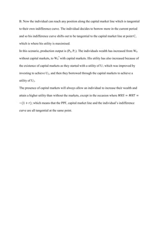
9. 3. If an individual has logarithmic utility and (Markowitz and cost of gamble) risk
premiafor the following gambles: (1) No initial wealth and gamble .8 prob. to obtain 10
and .2 prob. to obtain 40; (2) Current wealth 20 and gamble .1 prob. to obtain additional
20 and .9 prob. to obtain additional 90; (3) Current wealth 20000 and gamble .8 prob . to
lose 4000 and .2 prob. to lose 10000. Compare the two risk premia for each example.
i).
Current wealth=0
80% chance to gain £10
20% chance to gain £40
E(W)= 0.8*10+0.2*40= 16
E[U(W)]=0.8*ln(10)+0.2*ln(40)= 1.84+0.74=2.58
Wc= exp(2.58)= 13.20
W=E(W) because the expected change in wealth is zero.
Markowitz risk premium= E(W)-Wc=16-13.2=£2.80
Cost of gamble= W-Wc= 16-13.2=£2.80
Therefore there is no difference between the risk premium and the cost of gamble. As both
outcomes of the gamble are positive, this individual would be willing to pay up to £2.80 in
order to take this gamble.
ii).
Current wealth= £20
10% chance to gain +£20
90% chance to gain +£90
E(W)=0.1*20+0.9*90= 2+81= 83
E[U(W)]=0.1*[ln(20+20)]+0.9*[ln(20+90)]=4.60
Markowitz risk premium= 83-99.48= -£16.48
This individual would need to be paid £16.48 for him to not take the gamble.
Cost of gamble= 20 – 99.48= -£79.48
iii).
Current wealth= £20,000
80% chance to lose £4,000
20% chance to lose £10,000
E(W)= 0.8*16000+0.2*10000=14800.
E[U(W)]= 0.8*(ln16000)+0.2*(ln10000)=7.74+1.84=9.58
Markowitz risk premium= 14,800-14,472.42= £327.58.

10. This means that the individual would be willing to pay insurance against the gamble up to the
value of £327.58.
Cost of gamble= 20,000-14,472.42= £5,527.58.

11. 4. Show three alternative types of behaviour towards risk, by considering the shape of
the utility function as a function of wealth. What is a risk premium? How can be
approximated? (Please give no proofs.) Use indifference curves map of an individual in
mean (expected return) - standard deviation (risk) space to show risk aversion and risk
loving.
Assuming that marginal utility of wealth is positive, i.e. more wealth is better; there are three
types of behaviour a person can have towards taking risks.
The first type of behaviour is of risk lovers. This is shown by a convexed utility function, as
the individual’s utility of expected wealth will be lower than their expected utility of wealth.
These types of people love to take risks.
The second type of behaviour is of risk neutrality. This is characterised by a linear utility
function.This type of people are indifferent to taking risks.

12. The third type of behaviour is of a risk averter. This is shown by a concaved utility function,
as the individual’s utility of expected wealth will be greater than their expected utility of
wealth.These types of people are against risk taking behaviour.
A risk premium is the maximum amount of wealth that an individual would be willing to give
up in order to avoid a gamble. It is calculated by taking the difference between an
individual’s expected wealth when they take the gamble and the certainty equivalent wealth,
which is the level of wealth that an individual would accept with certainty if the gamble was
to be removed. Shown in mathematical form this looks like
The graph below shows an individual’s indifference curves in risk-return space when they
have the behaviour of a risk averter.

13. U4 U3 U2 U1
The indifference curves show all an individual’s combinations of risk and return that yield the
same expected utility of wealth.U1<U2<U3<U4 as the person is receiving the same amount of
return for less risk when comparing the indifference curves by expected return, i.e. increasing
utility.
The following graph now shows the indifference curves of an individual in risk-return space
when they are a risk lover.

14. U1<U2<U3<U4 as the person is receiving the same amount of return for more risk when
comparing the indifference curves by expected return, i.e. increasing utility.
5. Given the exponential utility function U(W) = -e-W
(i) Sketch a graph of the function.
(ii) Does the function exhibit positive marginal utility and risk aversion?
(iii) Does the function have decreasing absolute risk aversion?
(iv) Does the function have constant relative risk aversion?
i).

15. ii). Marginal utility can be derived by taking the first derivative of the utility function with
respect to Wealth.
Therefore, the function exhibits positive marginal utility. This is confirmed by the graph
above as the slope of any line which is tangent to the utility function at any point is always
positive.
To calculate whether the graph shows risk aversion, marginal utility must be differentiated to
find the rate of change in marginal utility.
The utility function therefore exhibits risk aversion, which is supported by analysing the
graph above which is concaved.
iii). The definition of Absolute Risk Aversion (ARA) is given by the equation
ARA measures risk aversion for a given level of wealth. Substituting in the values from the
previous part of the question can produce the ARA.
Therefore, this function does not have a decreasing ARA; instead it has a constant ARA.
iv). The equation for Relative Risk Aversion (RRA) is given by:
Then substituting in the values from the previous question the RRA can be calculated
Therefore, this utility function does not exhibit a constant relative risk aversion; instead
changes depending on wealth.

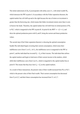
16. 6. A businessman faces a 10 % chance of having a fire that will reduce his net
wealth to £ 1, a 10 % chance that fire will reduce it to £ 100,000, and an 80 % chance
that nothing detrimental will happen, so that his business will retain its worth (£
200,000). What is the maximum amount he will pay for insurance if he has logarithmic
utility function U(W) = ln(W)? Explain your answer in detail.
Current wealth= £200,000
Gamble:
10% chance to be worth £1
10% chance to be worth £100,000
80% chance to be worth £200,000
E(W)= (0.1*1)+(0.1*100,000)+(0.8*200,000)= £170,000.10
E[U(W)]= (0.1*ln[1])+(0.1*ln[100,000])+(0.8*ln[200,000])=10.91615066
Wc = e10.91615066 = 55,058.45
The maximum risk premium that the business man is willing to pay is:
The Markowitz risk premium has been used to calculate the business man’s maximum risk premium
because by definition the Markowitz risk premium is the maximum amount of money that he would
pay to insure against the gamble. So this businessman is willing to pay an insurance premium up to
£114,941.55 to protect against fires.