Final Thesis Report

DESIGN AND IMPLEMENTATION OF A
“DIY” DIGITAL IMAGE CORRELATION
SYSTEM
Mr HJG Scotcher
23 October 2015

DESIGN AND IMPLEMENTATION OF A
“DIY” DIGITAL IMAGE CORRELATION
SYSTEM
MECHANICAL PROJECT 478
FINAL REPORT
Mr HJG Scotcher
Student no 17087996
Supervisor: Dr T Becker
23 October 2015

i
Executive Summary
Title of Project
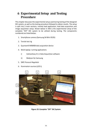
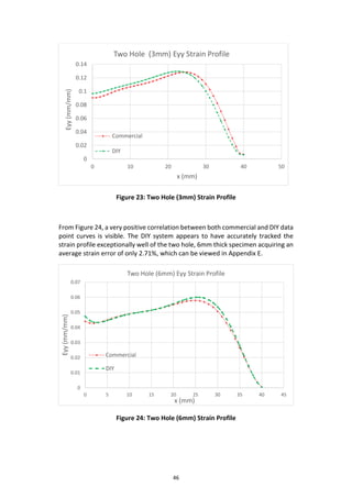
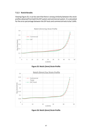
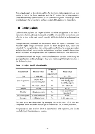
The design and implementation of a “DIY” Digital Image Correlation system
Objectives
Design and build a more cost-effective, simpler and technically sound DIC system using
cheaper and more readily available materials that will provide accurate results in the
area of full field surface measurements.
What aspects of the project are new/unique?
Formulating the design requirements for a cheaper, simple interface DIC system.
Commissioning the system through physical experiments to ensure it produces desired
results.
What are the expected findings?
Whether producing a “DIY” DIC system with more cost-effective materials and simpler
design that is suitable for 2D surface measurements will be feasible or not.
What value do the results have?
To provide a more economical alternative to conventional expensive DIC systems in the
aid of fracture mechanic research, and allow for ease of demonstration in the
classroom due to compact design
What contribution have/will other students made/make?
A previous student assisted in the configuration of an accurate and concise Matlab
based DIC algorithm that will be implemented in the design.
What aspects of the project will carry on after completion?
Redesign the pneumatic supply to exert incremental loading autonomously
What are the expected advantages of continuation?
Further exploration will aid in improving the system to be better implemented into daily
classroom use for the demonstration of fracture mechanics.
What arrangements have been made to expedite continuation?
The final design has been defined and recorded in sufficient detail to best allow
economic value and production demand analysis

ii
Plagiarism declaration
I know that plagiarism is wrong.
Plagiarism is to use another's work (even if it is summarised, translated or
rephrased) and pretend that it is one's own.
This assignment is my own work.
Each contribution to and quotation (e.g. "cut and paste") in this assignment from
the work(s) of other people has been explicitly attributed, and has been cited and
referenced. In addition to being explicitly attributed, all quotations are enclosed
in inverted commas, and long quotations are additionally in indented paragraphs.
I have not allowed, and will not allow, anyone to use my work (in paper, graphics,
electronic, verbal or any other format) with the intention of passing it off as his/her
own work.
I know that a mark of zero may be awarded to assignments with plagiarism and
also that no opportunity be given to submit an improved assignment.
I know that students involved in plagiarism will be reported to the Registrar and/or
the Central Disciplinary Committee.
Name: ........................................................
Student no: ........................................................
Signature: ........................................................
Date: ........................................................

iii
Outcome Sections in report
ELO 1. Problem solving: Demonstrate competence to
identify, assess, formulate and solve convergent
and divergent engineering problems creatively and
innovatively.
1; 2; 3; 4
ELO 2. Application of scientific and engineering
knowledge: Demonstrate competence to apply
knowledge of mathematics, basic science and
engineering sciences from first principles to solve
engineering problems.
5; 6; 7; Appendix D;
ELO 3. Engineering Design: Demonstrate competence
to perform creative, procedural and non-procedural
design and synthesis of components, systems,
engineering works, products or processes.
4; 5; 6; 7
ELO 5. Engineering methods, skills and tools,
including Information Technology: Demonstrate
competence to use appropriate engineering
methods, skills and tools, including those based on
information technology.
5; 6; 7; Appendix D;
Appendix E
ELO 6: Professional and technical communication:
Demonstrate competence to communicate
effectively, both orally and in writing, with
engineering audiences and the community at large.
Project Proposal;
Progress Report;
Progress Oral
Presentation; First
Report Draft; Final
Report; Project Poster
ELO 8. Individual, team and multi-disciplinary
working: Demonstrate competence to work
effectively as an individual, in teams and in
multidisciplinary
environments
4; 5
ELO 9. Independent learning ability: Demonstrate
competence to engage in independent learning
through well-developed learning skills.
1; 2; 4; 5; 6; MATLAB
skills

iv
ACKNOWLEDGEMENTS
The author would like to extend a special thanks to Dr. Thorsten Becker for his
clear guidance and support throughout the duration of the project. For final
prototype manufacture and continuous advice, the author would like to
specifically thank Mr Graham Hamerse, Mr Ferdi Zietsman and Mr Kobus
Zietsman.

v
Table of contents
Page
Executive Summary...........................................................................................i
Plagiarism declaration......................................................................................ii
Table of contents .............................................................................................v
List of Tables................................................................................................. viii
List of Figures..................................................................................................ix
Nomenclature.................................................................................................xi
1 Introduction..............................................................................................1
1.2 Objectives................................................................................................2
1.3 Motivation...............................................................................................2
1.4 Completed Activities ...............................................................................3
1.4.1 Identify Suitable Applications......................................................3
1.4.2 Compile System Design Requirements .......................................3
1.4.3 Concept Generation for the DIC system .....................................3
1.4.4 Detailed Concept Evaluation .......................................................3
1.4.5 Final Concept Selection ...............................................................3
1.4.6 Prototype Model Detail Design...................................................3
1.4.7 Concept Design Report................................................................4
1.4.8 Prototype Model Manufacturing ................................................4
1.4.9 Assembly Testing.........................................................................4
1.4.10 DIC System Validation .................................................................4
2 Literature Review......................................................................................4
2.1 Digital Image Correlation ........................................................................4
2.2 DIC System Components.........................................................................7
2.2.1 Tensile Testing Machine..............................................................7
2.2.2 Image Capture Device .................................................................9
2.2.3 Lighting ......................................................................................10
2.2.4 Data Acquisition ........................................................................11
2.3 Ncorr 2D DIC Matlab Program ..............................................................12
2.4 SU Materials Department DIC System ..................................................15
3 Problem Definition ..................................................................................16
3.1 Engineering Characteristics...................................................................16

vi
3.2 Product Design Specifications...............................................................17
4 Concept Generation ................................................................................18
4.1 System Decomposition..........................................................................18
4.2 Functional Structure..............................................................................20
4.3 Component Solution Concepts .............................................................20
4.4 Concept Evaluation and Selection.........................................................21
4.4.1 DIC Concept Feasibility Evaluation............................................21
5 DIC System Analysis.................................................................................23
5.1 Image Capture Device: Samsung I9195 S4 Mini Smartphone...............23
5.2 Tensile Test Mechanism........................................................................26
5.2.1 Force Application.......................................................................26
5.2.2 Specimen ...................................................................................27
5.3 Illumination Source ...............................................................................29
5.4 Data Capture/Acquisition......................................................................30
5.4.1 Load Data Capture.....................................................................30
5.4.2 Image Processing Software .......................................................33
5.5 Final Manufactured DIC Prototype .......................................................33
6 Experimental Setup and Testing Procedure.............................................35
6.1 System Experimental Setup ..................................................................36
6.1.1 Load Application Setup..............................................................36
6.1.2 Load Data Acquisition................................................................38
6.1.3 Image Acquisition Setup............................................................38
6.2 Testing Procedure .................................................................................38
7 Experimental Data Analysis .....................................................................41
7.1 Method of Analysis................................................................................41
7.2 Results and Findings..............................................................................43
7.2.1 One Hole Results .......................................................................43
7.2.2 Two Hole Results .......................................................................45
7.2.3 Notch Results.............................................................................47
8 Conclusion...............................................................................................48
9 Recommendations ..................................................................................49
10 Bibliography............................................................................................50
Appendix A Techno-Economic Analysis .......................................................52

vii
Appendix B Planned vs Actual Schedule......................................................55
Appendix C DATA SHEETS ...........................................................................56
Appendix D Experimental Testing Procedure...............................................59
Appendix E Strain Error Calculations...........................................................69

viii
List of Tables
Table 1: Design Parameters...................................................................................16
Table 2: Design Variables.......................................................................................16
Table 3: DIC System Specifications ........................................................................17
Table 4: Component Solution Concepts ................................................................21
Table 5: Feasible Concepts ....................................................................................22
Table 6: Configuration Design Specifications ........................................................22
Table 7: Specimen Design......................................................................................27
Table 8: Load cell wiring setup ..............................................................................32
Table 9: Manufactured Model Components .........................................................33
Table 10: Load Application Components...............................................................36
Table 11: DIY DIC Testing Specifications................................................................39
Table 12: Commercial DIC System Parameters .....................................................40
Table 13: Project Specification Checklist...............................................................48
Table 14: Budget Analysis of planned versus actual cost for engineering time....52
Table 15: Budget Analysis of planned versus actual material costs.....................53
Table 16: Pre-test Apparatus.................................................................................59
Table 17: One Hole (3mm) Error............................................................................69
Table 18: One Hole (6mm) Error............................................................................70
Table 19: Two Hole (3mm) Error ...........................................................................71
Table 20: Two Hole (6mm) Error ...........................................................................72
Table 21: Notch (3mm) Error.................................................................................73
Table 22: Notch (6mm) Error.................................................................................74

ix
List of Figures
Figure 1: Point Transformation (Tang, et al., 2012).................................................6
Figure 2: Deformation Mapping (M.R. Maschmann, 2012) ....................................6
Figure 3: MTS Criterion Series 40 (Corporation, 2015) ...........................................8
Figure 4: Specimen Grip Summary (Albert, 2014)...................................................9
Figure 5: DIC lighting source ..................................................................................11
Figure 6: Ncorr subset coordinates (Blaber, 2015)................................................12
Figure 7: Mechanical Department LaVision DIC System .......................................15
Figure 8: DIC Physical Decomposition ...................................................................18
Figure 9: DIC Functional Structure.........................................................................20
Figure 10: Samsung I9195 S4 Mini.........................................................................23
Figure 11: Norgren RT/57220/M50 .......................................................................26
Figure 12: Stress factor Kt of hole specimen .........................................................28
Figure 13: Specimen Clamp Force Diagram...........................................................29
Figure 14: Illumination Angle.................................................................................30
Figure 15: Loading Force Diagram .........................................................................31
Figure 16: HBM QuantamX MX840B .....................................................................31
Figure 17: Load cell wiring diagram.......................................................................32
Figure 18: Final manufactured DIC prototype.......................................................34
Figure 19: Complete "DIY" DIC System..................................................................35
Figure 20: Force Application Assembly..................................................................37
Figure 21: One Hole (3mm) Strain Profile..............................................................44
Figure 22: One Hole (6mm) Strain Profile..............................................................45
Figure 23: Two Hole (3mm) Strain Profile .............................................................46
Figure 24: Two Hole (6mm) Strain Profile .............................................................46
Figure 25: Notch (3mm) Strain Profile...................................................................47
Figure 26: Notch (6mm) Strain Profile...................................................................47
Figure 27: Tubing Schematic..................................................................................60
Figure 28: Pneumatic Supply Lever .......................................................................61

x
Figure 29: Festo Pneumatic Supply Gauge ............................................................61
Figure 31: Smartphone camera mounted .............................................................62
Figure 32: TimeLapse Pro Capture.........................................................................63
Figure 33: Ncorr GUI ..............................................................................................65
Figure 34: ROI Draw Method.................................................................................66
Figure 35: Strain Parameters GUI ..........................................................................68

xi
Nomenclature
COMMON ACRONYMS
DIC Digital Image Correlation
CCD Charge-Coupled Device
CMOS Complementary Metal-Oxide Semiconductor
FOV Field-of-View
DOF Depth-of-Field
GUI Graphic User Interface
DIY Do-It-Yourself

1
1 Introduction
The concept and application of digital image correlation (DIC) has been evident
since approximately 1975, with greater emphasis on its optimization occurring in
recent years. Present DIC systems are used frequently in laboratory research in
the field of fracture mechanics and material property testing, but are currently
highly expensive, and are not easily transported due to their bulky dimensions.
The need exists for a more compact, cost-effective DIC system with a simpler user-
interface.
The project given is a study into the design and implementation of a single-camera
“Do-It-Yourself” (DIY) DIC system that will be suitable for simpler user-interface
and integrated classroom demonstrations. Factors such as production cost will
play a role in the design, but the primary focus of the thesis will be to produce a
more compact and simplified DIC system. This study, which Mr HJG Scotcher is
doing as part of Mechanical Project 478, stems from a proposal put forth by Dr T
Becker.
The proposed design will be suitable for interactive classroom demonstrations,
along with performing accurate digital image correlation on a variety of materials
in order to obtain full field strain maps. Non-destructive-testing (NDT) has become
a viable way of obtaining new information pertaining to the material properties of
an array of substances.
This report documents the project’s objectives, motivation and planning. Initially
identifying certain concepts, this report discusses and presents a detailed
prototype design, followed by experimental testing and results discussion. The
report takes into account time, cost and feasibility purposes of the design and
implementation of the proposed system.
The overall purpose of this report is to present a more portable, cost-effective DIC
system capable of producing results within a specified error region of conventional
systems.

2
1.2 Objectives
As shown above, this project is centred on the design and implementation of a “DIY”
DIC system. The objectives of this study are as follows:
2.1 Conduct a thorough literary review to provide suitable background to the given
project, as well as providing information for innovation.
2.2 Designing the system to be composed of cost-effective, alternative components
whilst still producing accurate results.
2.3 Designing the system to operate with a simpler user-interface than current
commercial models.
2.4 Selecting suitable components to ensure a compact design for easy
transportation, set-up and installation by a single person.
2.5 Validate and commission the designed system through detailed testing and
analysis
1.3 Motivation
Current DIC systems provide detailed and expansive results pertaining to the area
of fracture mechanics, but commercial systems are not only highly expensive, but
also too bulky for easy disassembly and assembly. To reduce the cost whilst
ensuring a more compact, and simpler form of a DIC system will benefit areas at
both university and industry level. The use of this more compact system in the
teaching environment will aid students in their understanding of fracture
mechanics, whilst use in industry will allow for faster, more cost-effective
preliminary sample testing to take place. The Department of Mechanical and
Mechatronic Engineering has multiple resources available to aid this study,
including current commercial DIC systems to be used for benchmarking purposes,
and a multitude of existing knowledge pertaining to the field of DIC.

3
1.4 Completed Activities
The following activities have been completed thus far in the project.
1.4.1 Identify Suitable Applications
Research and identify those applications most suited to the design and
implementation of a “DIY” DIC system, and which applications will most
benefit from the implementation of such a system.
1.4.2 Compile System Design Requirements
Identification and selection of design requirements suited to ensure
optimization of the DIC system in selected applications. The complete life
cycle of the DIC system will be taken into consideration to ensure all facets
are accounted for. This will include initial concept generation, system
development and commissioning, operation and maintenance.
1.4.3 Concept Generation for the DIC system
Generate a number of feasible concepts based on requirements listed in the
previous activity, as well as ensuring each concept meets previously listed
objectives. Formulate a set of evaluation criteria on which to judge each
individual concept. Document final assessments of all concepts for later
review to aid in design improvement.
1.4.4 Detailed Concept Evaluation
Investigate each individual concept in detail to assess possible advantages
and shortcomings, and whether various facets from multiple concepts may
be combined. Detailed concept review to assess to what extent each
concept meets given design requirements.
1.4.5 Final Concept Selection
Utilize information extracted from previous activity to make a final and
wholly motivated decision of final concept suited to fulfil design
requirements.
1.4.6 Prototype Model Detail Design
Design a detailed “DIY” DIC system based on the selected concept from the
previous activity. The design will be undertaken to ensure all listed

4
objectives will be achieved, including the planning of a suitable test
procedure to assess the final model.
1.4.7 Concept Design Report
Present proposed concept detail design to study supervisor to acquire
approval and possible improvements for selected concept.
1.4.8 Prototype Model Manufacturing
Send in necessary detailed drawings of devised rig/set-up to workshop to be
manufactured. Order all necessary “outside” components required for final
prototype.
1.4.9 Assembly Testing
Preliminary testing completed on individual sub-assemblies of the system
to ensure all facets of the design are working on their own before being
assembled into a single, cohesive unit.
1.4.10 DIC System Validation
Designed and built system has been tested and validated, using
Stellenbosch University Materials Laboratory DIC System for benchmarking
purposes.
2 Literature Review
The following chapter discusses and reviews information pertaining to the given
project, including past research on digital image correlation and information
related to the given project.
2.1 Digital Image Correlation
The fundamental approach to digital image correlation (DIC) involves the
comparison, or correlation, of two or more images of a single sample before and
after loading (Solutions, 2015). This correlation provides the user with full field 2D
and 3D deformation vector fields and strain maps. The most common form of
loading utilized is tension as this removes the complication of out-of-plane
deformation.

5
DIC has proven to be a more cost-effective and simpler method of strain
measurement than other techniques such as speckle interferometery, and has
shown to be a more accurate than manual methods of measurement such as
extensometers. DIC is most suited to applications such as crack propagation
measurement and situations in which a full field deformation map is required.
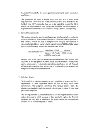
(Solutions, 2015)
Interest in DIC has grown over the past few years due to a number of reasons, the
main cause being the rapid improvement of charge-coupled device (CCD) and
complementary metal-oxide-semiconductor (CMOS) sensor-based cameras whilst
cost of these devices has decreased substantially. The dynamic range of these
cameras has allowed for a multitude of possible applications. Dynamic range is
measured in bit depth, which is defined as the number of bits of information in a
single sample and is directly related to resolution of each sample (DALSA, 2015).
Modern cameras generally have a bit size varying from 8 to 14-bit and it is this
improved resolution that has driven the movement towards greater DIC use.
A complete DIC system consists of 3 main components, namely a loading
mechanism, image capture device and some form of image acquisition and
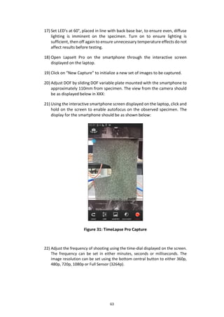
processing station. Common DIC systems make use of a tensile testing machine as
the loading mechanism, but compression machines can be used if needed. Image
acquisition and processing is achieved through the implementation of high-speed
correlation software. A large number of software packages are available, but all
software tends to utilize similar correlation algorithms.
The correlation algorithm is utilized by having the software initially divide the
chosen field-of-view (FOV) into a number of smaller subsections, called subsets
(Yoneyama & Murasawa, 2013). These subsets are essentially a group of random
coordinate points. As the specimen undergoes loading, these various subsets
undergo a spatial transformation. DIC commonly makes use of a function known
as the correlation coefficient, and is shown in equation 2.1.
𝑟𝑖𝑗 (𝑢, 𝑣,
𝜕𝑢
𝜕𝑥
,
𝜕𝑢
𝜕𝑦
,
𝜕𝑣
𝜕𝑥
,
𝜕𝑣
𝜕𝑦
) = 1 −
∑𝑖∑ 𝑗[𝐹(𝑥 𝑖,𝑦 𝑗)−𝐹̅][𝐺(𝑥 𝑖
∗
,𝑦 𝑗
∗
)−𝐺̅]
√∑𝑖∑ 𝑗[𝐹(𝑥 𝑖,𝑦 𝑗)−𝐹̅]
2
∑𝑖∑ 𝑗[𝐺(𝑥 𝑖
∗,𝑦 𝑗
∗)−𝐺̅]
2
(2.1)
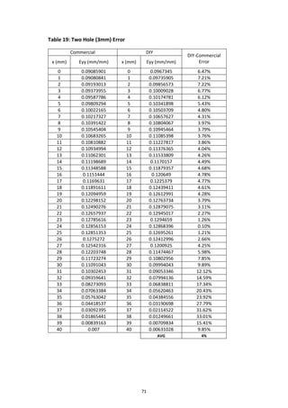
In this equation, F(xi,yj) is the grey scale value at a point (xi,yj) in the initial
reference image and G(xi*,yj*) is the grey scale value at a point (xi*,yj*) in the
following, deformed image. 𝐹̅ and 𝐺̅ are the mean values of the gray scale values
of matrices F and G, respectively (H.A. Bruck, 1989). This equation is relatively
complicated and for 2D DIC the relation between (xi,yj) and (xi*,yj*) can be
approximated as a linear, first order transformation equation as shown below in
equation 2.2 and 2.3:

6
𝑥∗
= 𝑥 + 𝑢 +
𝜕𝑢
𝜕𝑥
∆𝑥 +
𝜕𝑢
𝜕𝑦
∆𝑦 (2.2)
𝑦∗
= 𝑦 + 𝑣 +
𝜕𝑣
𝜕𝑥
∆𝑥 +
𝜕𝑣
𝜕𝑦
∆𝑦 (2.3)
A graphical representation of the transformation of points x and y are shown in
Figure 2.1. In this linear approximation, u and v are the translations of the central
point of the subset in the X and Y directions, respectively. The distance travelled
by each x and y coordinate to the current configuration are denoted as Δx and Δy,
respectively. This linear approximation is commonly referred as phase correlation.
Phase correlation is significantly faster, as it does not directly analyse the
correlation coefficient. (H.A. Bruck, 1989)
Figure 1: Point Transformation (Tang, et al., 2012)
From the calculated transformations of a certain number of continuous subsets,
full field displacement maps can be generated along with closely approximated
strain measurements. A graphical representation of deformation mapping is
shown in figure 2.
Figure 2: Deformation Mapping (M.R. Maschmann, 2012)

7
Commercial DIC systems implement extensive and complicated correlation
programs that require induction training in order to use. Simpler correlation
programs are available through open source software, software easily
implemented and user-friendly. One of the leading software algorithms for DIC
freely available online is Ncorr 2D DIC MATLAB program.
2.2 DIC System Components
Commercial DIC systems consist of an assembly of separate components all
operating in conjunction with one another to produce accurate strain
measurement results. Accuracy achieved for DIC purposes greatly depend on the
choice of components implemented within the proposed system. This section
focuses on the components typically implemented within conventional DIC
systems.
2.2.1 Tensile Testing Machine
Tensile testing is defined as the method of exerting a tensile, or pulling, force on
an object such that it undergoes axial elongation (Gharagozlou, 2014). Commercial
tensile machinery are split into two main categories, namely electro-mechanical
and hydraulic systems. A number of other load application mechanisms do exist,
but these are the methods most often used alongside DIC.
Electromechanical systems are well suited to low- to medium force testing
applications, readily used for their superior reliability in high-speed, low vibration
testing conditions. These systems, such as the MTS Criterion Series 40 shown
below in Figure 3, generally consist of a compact, 2-column frame configuration,
a high resolution load cell and compatible software for user control over selective
testing conditions.

8
Figure 3: MTS Criterion Series 40 (Corporation, 2015)
The compact AC servomotor built into the base of the frame drives two ball screws
mounted within a crosshead. This translates rotational motion into linear
movement, causing the crosshead to exert a tensile force onto the clamped
specimen. High-resolution digital controllers deliver high-speed, closed-loop
control able to achieve a data acquisition rates up to 1000 Hz, able to generate
detailed data for more accurate analysis (Corporation, 2015).
Hydraulic systems differ quite greatly from electromechanical systems, and make
use of hydraulic cylinder pressure for medium- to high load exertion up to 2000
kN. (Gharagozlou, 2015). Advanced hydraulic system control allow for high
precision pressure regulation during testing.
Clamping methods used in tensile testing play an important role in ensuring all
stress developed within the specimen due to imposed tensile load is isolated to
the observable area. The specimen under testing is firmly held between two
clamps, utilizing normal and frictional forces to hold the specimen in place. The
choice of clamp is specific to the specimen design and material used. There are a
number of available options for clamps, many of which are interchangeable with
standard tensile testing machines.
There are two main categories of clamps specific to tensile testing, namely positive
clamping and non-positive clamping types. A summary of both of these categories
as well as the various grips associated with each is shown in figure 3. Positive
clamping requires no additional forces as the specimen is gripped via a form fit
and this type is usually associated with conical shaped specimens. Non-positive
clamping requires the addition of a frictional force to ensure the specimen does
not slip from the grip. ( (Albert, 2014)

9
Figure 4: Specimen Grip Summary (Albert, 2014)
2.2.2 Image Capture Device
As stated above, large advances have been made with regards to the digital
cameras utilized with commercial DIC systems. The improvements in this area has
made DIC a more favourable form of displacement tracking and strain
measurement.
These cameras typically make use of either a charge-coupled device (CCD) or
complementary metal-oxide-semiconductor (CMOS) based sensor. (DALSA,
2015).These sensors work by converting the light that strikes the face of each
individual cells into an electronic signal. Each sensor is made up of a large number
of these cells, and each cell acts by converting the incident light into a small
electrical charge. These charges are converted to a voltage one pixel at a time as
they are read from the chip, and together they produce an image of high-
resolution and low-noise.
There are number of differences between CCD and CMOS sensors, and careful
consideration should be taken when selecting a sensor for a specific application.
CMOS sensors are more susceptible to noise than CCD sensors, but have an
advantage in being far more inexpensive as they can be fabricated on any standard
silicon production line. The reason for the increased cost of CCD sensors lies in
their ability to transport charge across the individual chips without distortion.
CMOS sensors undergo similar manufacturing processes used to make
microprocessors, whilst CCD sensors require special fabrication to remove the
distortion through transport.

10
An important value to look at when selecting the sensor type to utilize is the size
of pixel generated. Pixel size of camera lenses greatly impact the spatial resolution,
defined as the extent of the sensors ability to capture small detail. Therefore a
smaller pixel size correlates to greater resolution, whilst a larger pixel size tends
to reduce image noise. Pixel size range between 1 and 6 µm have been proven to
produce image resolution suitable for accurate image correlation. Pixel size of a
sensor can be calculated as shown below:
𝑷𝒊𝒙𝒆𝒍 𝒔𝒊𝒛𝒆 =
𝒔𝒆𝒏𝒔𝒐𝒓 𝒘𝒊𝒅𝒕𝒉
𝒉𝒐𝒓𝒊𝒛𝒐𝒏𝒕𝒂𝒍 𝒑𝒊𝒙𝒆𝒍 𝒒𝒖𝒂𝒏𝒕𝒊𝒕𝒚
(1)
Apart from sensor type, another important facet of camera selection is the lens
used during capture. Certain factors influence the type of lens selection suitable
for a specific testing environment (Sutton, et al., 2009) . These factors include:
1) Field-Of-View (FOV): visible image area captured by the lens (height x
width)
2) Depth-Of-Field (DOF): distance from lens to observable specimen
3) Sensor size: physical dimensions of camera CCD/CMOS sensor
These factors all directly influence one another, and selection of lens suitability
depends on the values desired for each factor. Selection of preliminary values for
these factors allows the user to calculate the required focal length for imaging
camera shown below:
𝑭𝒐𝒄𝒂𝒍 𝒍𝒆𝒏𝒈𝒕𝒉 =
𝑺𝒆𝒏𝒔𝒐𝒓 𝒔𝒊𝒛𝒆∗𝑫𝑶𝑭
𝑭𝑶𝑽
(2)
Once estimate focal length has been obtained, and suitable lens selection has
been made, rearranging the above formula provides a means to see how altering
the distance of lens to specimen affects the FOV captured by the camera:
𝑭𝑶𝑽 =
𝑺𝒆𝒏𝒔𝒐𝒓 𝒔𝒊𝒛𝒆∗𝑫𝑶𝑭
𝑭𝒐𝒄𝒂𝒍 𝒍𝒆𝒏𝒈𝒕𝒉
(3)
2.2.3 Lighting
For accurate and constant image capture to occur, the specimen under observation is
subjected to a high intensity white light in order to reduce the effects of decorrelation
caused by varying ambient light. Conventional DIC systems commonly implement
two LED lighting sources of varying sizes and shapes.

11
The LED’s used ensure sufficient image contrast, emitting mid-wavelength light of
450 nm from varying orientations to provide even and and stable lighting. The
camera is often fitted with a specific optical bandpass filter. These filters allow for
only light within a specified range (ie 428-470nm) to pass through, effectively
eradicating the effect of lighting outside this range from reaching the camera
sensor. If a filter is used, the resulting image is of low intensity and high contrast
as only limited light within the bandpass range can pass through the sensor.
Typical lighting sources used within DIC is shown below in Error! Reference source
ot found..
Figure 5: DIC lighting source
The LED’s commonly used are not constantly active throughout testing, as the heat
radiation emitted from them can have resulting effects on the specimen under
observation due to temperature increases. Thus a means to emit light at
predefined intervals of image capture are required. To accomplish this, a data
acquisition controller that allows for high accuracy trigger control is utilized,
having both optical camera’s and lighting sources digitally connect via data cables
to ensure images are taken in precise timing with LED illumination. This on/off
lighting system thus ensures not only high contrast image quality, but isolates the
effect of thermal radiation and temperature effects on strain readings.
2.2.4 Data Acquisition
Successful DIC strain readings require accurate and synchronized data and image
acquisition. This synchronization is achieved through the implementation of a data
acquisition central control unit. The control unit coordinates all devices and
sensors connected to it via digital data cables, and is completely operable through
associated DIC software.
The software allows for complete control over all settings pertaining to connected
sensors and illumination devices, providing versatility to handle a number of
various testing procedures and situations. DIC software not only allows for control

12
over these physical devices, but also incorporates the ability to maintain total
control over post-processing, data analysis and management. The software is
installed into a standard PC/laptop connected to the central control unit via a high
speed Universal Serial Bus (USB) for fast data transfer between devices and
software.
Conventional DIC systems are sold as a total package, including optical camera’s,
illumination sources, central data control unit and associated software, done so to
remove any compatibility issues that may arise through the grouping of external
devices and software.
2.3 Ncorr 2D DIC Matlab Program
Ncorr offers an open source 2D digital image correlation MATLAB program, and is
fully operable through an accessible and simple graphic user interface (GUI). The
program provides the user with a means to process images to produce detailed
displacement and strain fields within a selected region of interest (ROI) for a given
sample under testing (Blaber, 2015).
The program operates similar to conventional DIC software such as DaVis and VIC-
3D, utilizing the grouping of coordinate points into subsets and the movement
they undergo during testing to calculate full field strain maps. The procedure by
which Ncorr processes these subsets is shown in Figure 6 below:
Figure 6: Ncorr subset coordinates (Blaber, 2015)
Transformation of initial reference subset points to current position is simplified
from the conventional correlation coefficient as discussed in Section XX by
constraining the motion to a linear, first order transformation as shown below:

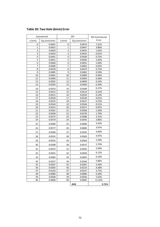
13
𝒙 𝒄𝒖𝒓,𝒊 = 𝒙 𝒓𝒆𝒇,𝒊 + 𝒖 𝒓𝒄 +
𝝏𝒖
𝝏𝒙 𝒓𝒄
(𝒙 𝒓𝒆𝒇,𝒊 − 𝒙 𝒓𝒆𝒇,𝒄) +
𝝏𝒖
𝝏𝒚 𝒓𝒄
(𝒚 𝒓𝒆𝒇,𝒊 − 𝒚 𝒓𝒆𝒇,𝒄) (4)
𝐲𝒄𝒖𝒓,𝒊 = 𝐲𝒓𝒆𝒇,𝒊 + 𝐯𝒓𝒄 +
𝝏𝒗
𝝏𝒙 𝒓𝒄
𝝏𝒗
𝝏𝒚 𝒓𝒄
𝑥 𝑟𝑒𝑓,𝑖 and 𝑦 𝑟𝑒𝑓,𝑖indicate the x and y coordinates of an initial reference subset point,
𝑥 𝑟𝑒𝑓,𝑐 and 𝑦 𝑟𝑒𝑓,𝑐 the x and y coordinates of the center of the initial reference
subset and 𝑥 𝑐𝑢𝑟,𝑖 and 𝑦𝑐𝑢𝑟,𝑖 the x and y coordinates of the final current subset
point. (i,j) coordinates are used to indicate a relevant location of subset points
with respect to the center of the subset. The subscript “rc” indicates the
transformation from the reference to the current coordinate system (Blaber,
2015).
A deformation vector, p, is defined below as column vector of all transformation
functions:
𝒑 = { 𝒖 𝒗
𝝏𝒖
𝝏𝒙
𝝏𝒖
𝝏𝒚
𝝏𝒗
𝝏𝒙
𝝏𝒗
𝝏𝒚
} 𝑻
(6)
Equation 4 and 5 can be written into matrix form, where ξ is an augmented vector
containing the x and y coordinates of subset points, Δx and Δy the distances
between a subset point and the center of the subset, and “w” defined as function
called a warp. The matrix form is shown below:
𝝃 𝒓𝒆𝒇,𝒄 + 𝒘(𝜟𝝃 𝒓𝒆𝒇, 𝒑 𝒓𝒄) = {
𝒙 𝒓𝒆𝒇,𝒄
𝑻
𝒚 𝒓𝒆𝒇,𝒄
𝑻
𝟏
} +
[
𝟏 +
𝒅𝒖
𝒅𝒙 𝒓𝒄
𝒅𝒖
𝒅𝒚 𝒓𝒄
𝒖 𝒓𝒄
𝒅𝒗
𝒅𝒙 𝒓𝒄
𝟏 +
𝒅𝒗
𝒅𝒚 𝒓𝒄
𝒗 𝒓𝒄
𝟎 𝟎 𝟏 ]
∗ {
𝜟𝒙 𝒓𝒆𝒇
𝑻
𝜟𝒚 𝒓𝒆𝒇
𝑻
𝟏
} (7)
For computational purposes, the reference subset is allowed to deform within the
reference configuration as shown below:
𝒙 𝒏𝒆𝒘𝒓𝒆𝒇,𝒊 = 𝒙 𝒓𝒆𝒇,𝒊 + 𝒖 𝒓𝒓 +
𝝏𝒖
𝝏𝒙 𝒓𝒓
(𝒙 𝒓𝒆𝒇,𝒊 − 𝒙 𝒓𝒆𝒇,𝒄)
+
𝝏𝒖
𝝏𝒚 𝒓𝒓
𝒚 𝒏𝒆𝒘𝒓𝒆𝒇,𝒋 = 𝒚 𝒓𝒆𝒇,𝒊 + 𝒗 𝒓𝒓 +
𝝏𝒗
𝝏𝒙 𝒓𝒄
𝝏𝒗
𝝏𝒚 𝒓𝒄

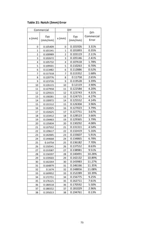
14
𝑥 𝑛𝑒𝑤𝑟𝑒𝑓,𝑖 and 𝑦 𝑛𝑒𝑤𝑟𝑒𝑓,𝑗 are the x and y coordinates of a final reference subset. The
use of the “rr” subscript is to indicate transformation from the reference
coordinate system to the reference coordinate system. For the computational
purposes, is desired to find the optimal prc, when prr = 0, such that the coordinates
at 𝒙 𝒏𝒆𝒘𝒓𝒆𝒇,𝒊 and 𝑦 𝑛𝑒𝑤𝑟𝑒𝑓,𝑗 are approximately equal to the coordinates at
𝑥 𝑐𝑢𝑟,𝑖 andy 𝑐𝑢𝑟,𝑖 .
The program is similar to conventional systems in using correlation criteria, a
means to establish a metric for similarity between the final reference subset and
the final current subset. The program does so by comparing grayscale values at
the final reference subset points with grayscale values at the final current subset
points. The two equations implemented within the program are shown below:
𝑪 𝒄𝒄 =
𝜮(𝒊,𝒋)(𝒇(𝒙 𝒏𝒆𝒘𝒓𝒆𝒇,𝒊 ,𝒚 𝒏𝒆𝒘𝒓𝒆𝒇,𝒋)−𝒇 𝒎)(𝒈(𝒙 𝒄𝒖𝒓,𝒊,𝒚 𝒄𝒖𝒓,𝒋)−𝒈 𝒎)
√ 𝜮(𝒊,𝒋)[𝒇(𝒙 𝒏𝒆𝒘𝒓𝒆𝒇,𝒊,𝒚 𝒏𝒆𝒘𝒓𝒆𝒇,𝒋)−𝒇 𝒎]
𝟐
𝜮(𝒊,𝒋)[𝒈(𝒙 𝒄𝒖𝒓,𝒊,𝒚 𝒄𝒖𝒓,𝒋)−𝒈 𝒎] 𝟐
(10)
𝑪 𝑳𝑺 = 𝜮(𝒊,𝒋) [
𝒇(𝒙 𝒏𝒆𝒘𝒓𝒆𝒇,𝒊 ,𝒚 𝒏𝒆𝒘𝒓𝒆𝒇,𝒋)−𝒇 𝒎
√ 𝜮(𝒊,𝒋)[𝒇(𝒙 𝒏𝒆𝒘𝒓𝒆𝒇,𝒊,𝒚 𝒏𝒆𝒘𝒓𝒆𝒇,𝒋)−𝒇 𝒎]
𝟐
−
𝒈(𝒙 𝒄𝒖𝒓,𝒊,𝒚 𝒄𝒖𝒓,𝒋)−𝒈 𝒎
√𝜮(𝒊,𝒋)[𝒈(𝒙 𝒄𝒖𝒓,𝒊,𝒚 𝒄𝒖𝒓,𝒋)−𝒈 𝒎] 𝟐
] 𝟐
(11)
The formulas f and g indicate the reference and current image functions,
respectively, and return a grayscale value corresponding to the specified (x,y)
point. The grayscale values of the final reference and current subset are defined
as fm and gm respectively, and are shown below in the following equations:
𝑓𝑚 =
𝛴(𝑖,𝑗) 𝑓(𝑥 𝑛𝑒𝑤𝑟𝑒𝑓,𝑖, 𝑦 𝑛𝑒𝑤𝑟𝑒𝑓,𝑗)
𝑛(𝑆)
𝑔 𝑚 =
𝛴(𝑖,𝑗) 𝑔(𝑥 𝑐𝑢𝑟,𝑖, 𝑦𝑐𝑢𝑟,𝑗
𝑛(𝑆)
Where n(S) is the number of elements in S, the set which contains all the subset
points.

15
2.4 SU Materials Department DIC System
Stellenbosch University’s dedicated Materials Department has ownership of a
standard, high-quality DIC system. The system is utilized to perform digital image
correlation on a number of varing materials and specimen designs.
The setup, purchased from LaVision, consists of a stero vision camera setup to
accommodate for in-plane and out-of-plane measurements. The system is coupled
with an MTS Criterion Model 40 tensile testing machine as shown previously, and
offers a wide range of available scientific camera’s and lenses to allow for greater
diversity of specimen testing. The system utilizes LaVisions DaVis 8.2.3 DIC
software to aid in setup, testing and post-processing. A high-speed digital control
box ensures consistent and accurate triggering of camera shutters and
illumination to produce high-resolution images suitable for pixel correlation.
The system can provide as an authenticated means upon which to benchmark
other forms of strain measurement, and is depicted below in Figure 7:
Figure 7: Mechanical Department LaVision DIC System

16
3 Problem Definition
3.1 Engineering Characteristics
Listed below in Table 1 are the chosen design parameters for the proposed DIC
system. They are the physical guidelines on which the design is based.
Table 1: Design Parameters
Requirement Description Quantification
Size
The entire system is to be mobile
and small enough to fit on a
standard work desk.
< 0.8 x 0.5 x 0.5 m^3
Weight
The complete model is to be light
enough to be lifted by a single
person.
< 7 kilograms
Accuracy
The system is to product results
suitable for complete
deformation mapping
< 0.05 pixel error
Set-up
The system is to incorporate a
simple and fast set-up and
installation
< 5 sub-assemblies
Structural
Rigidity
The structure is to be structurally
sound with minimal allowable
movement and vibration
< 1 mm defection
Design variables given below in Table 2 highlight the areas of the design over which
the student has a choice. The given variables are key components of the design
and careful consideration must be taken with the final selection of each element.
Table 2: Design Variables
Requirement Description
Force Application
The device or method of force application is to impose a
steady and constant load on the specimen.
Image Capture Device
The choice of camera is to capture images whose quality is
suitable for image correlation
Specimen Material
The choice of material is to produce deformations suitable
for image correlation.

17
3.2 Product Design Specifications
The complete product design specifications are listed below in Table 3. These
specifications provide clear goals upon which the design can be based. It provides
a structure in which to design various feasible DIC system concepts.
Table 3: DIC System Specifications
Specification Quantity/Unit Description
Cost < R400 000
The total cost of all components, materials
and labour used within the given system is
to be less than commercial system cost.
Ease of
Operation
-
The proposed system is to incorporate a
simpler user-interface than current
commercial systems
Size
< 0.8 x 0.8 x
0.5 m
The entire system is to be suitable for
classroom demonstrations and able to fit
onto a standard work desk
Weight < 10 kg
The system is to be light-weight and easily
transported by a single person.
Modular
< 5 sub-
assemblies
The system is to be portable, and able to
be disassembled and transported to
another location with ease.
Structural
Rigidity
< 1mm
deflection
The frame is to undergo little, if any,
deformation due to testing or vibrations.
Accuracy
< 0.0.5 pixel
error
The proposed system is to achieve results
within an accuracy range suitable for full
field displacement and strain mapping.

18
4 Concept Generation
4.1 System Decomposition
Breaking the proposed DIC system down into its subsidiary sub-assemblies and
components allows for broad and explorative concept generation. The physical
breakdown of a conventional DIC system is shown below in Figure 8, and
provides for expansive consideration of possible system components.
Figure 8: DIC Physical Decomposition
From the above figure, it can be seen there are 4 core components that make up
the given DIC system. Each component to be selected requires to exhibit certain
qualities to meet the project objectives. The individual requirements of each
component have been listed below:
1.1 Image Capture Device
- Small pixel size ( < 5 µm )
- Time dependant capture method

19
- Low frame rate frequency ( <0.5 Hz )
- Tethering control via work laptop
- Cost-effectivity ( < R2000
1.2 Tensile Test
- Steady loading rates
- Good clamping mechanism
- Load cell accommodation
- Simple design
- Steady material deformation
- Lightweight structure
1.3 Lighting
- Produce diffuse light on specimen
- Cost effective
- Lightweight
1.4 Data Capture Device
- High resolution
- High data acquisition rate
- Low level percentage

20
4.2 Functional Structure
The functional structure, otherwise known as systematic design, provides a way
to describe an entire system in the form of labelled function blocks, and the way
in which they interact with one another via flow lines. Shown below is a graphical
function structure of the proposed DIC system.
Figure 9: DIC Functional Structure
4.3 Component Solution Concepts
Reviewing the individual components associated with the complete DIC system,
as well as the way in which each component interacts with the rest of the system
allows for investigative concept generation. A number of concepts exist for each
individual piece, but a large focus must be placed on the feasibility of these
components interacting with the rest of the system.
Shown below in Table 4 are a list of possible concepts for each component.
Depicting these available choices in such a way provides an approach to combine
components in a large range of alternative designs and assessing the feasibility
and viability of each combined system.

21
Table 4: Component Solution Concepts
Component Concept 1 Concept 2 Concept 3 Concept 4
1.1 Image Capture
Device
DSLR Camera
Hand-Held
Camera
Smartphone Web-Cam
1.2 Tensile Test
1.2.1 Specimen
Material
Perspex Natural Rubber LDPE Cardboard
1.2.2 Specimen Clamp
Mechanical
Wedge Action
Hydraulic
Actuated
In-house Design
1.2.3 Force
Application
Thread Screw
(Thrust
Bearing)
Lead Screws
(Actuator-
driven)
Pneumatic
Pistons
1.3 Lighting Wired LED's
Stand-alone
LED's
Monochromatic
lighting
1.4 Data Capture
Laptop
(MATLAB)
Micro-
processor
The above listed component concepts can now be assembled and constructed into
a variety of viable preliminary concept designs, with careful consideration to the
advantages and disadvantages of individual component concepts.
4.4 Concept Evaluation and Selection
This section dictates feasible concepts in their initial fabrication, and then
evaluation and final selection of a single model for further detail design.
4.4.1 DIC Concept Feasibility Evaluation
The concepts proposed above are fabricated together within a selection of
possible structural frames. These preliminary concepts are shown below in Table
5, and are suitable for evaluation and final selection.

22
Table 5: Feasible Concepts
Concept 1 Concept 2 Concept 3
Screw Thread Forcing
Mechanism (Thrust bearing; L-
Shape Adjustable Camera
Mount; Hand-Held Camera;
Lead Screw with Motor
Driven Actuator; Set
Camera Position;
Adjustable Webcam
Pneumatic Cylinder Forcing
Mechanism; Horizontal
Sliding Camera Mount;
Smartphone
Each concept is associated with its own set of advantages and disadvantages.
These factors play a major role in selecting and developing a fully functioning DIC
testing apparatus, a system that is capable of repeatedly producing desired
correlation results. Final selection of concept 3 was decided upon for overall
simplistic design, and ease of use. The motivation for each component is discussed
in Section 5.
Table 6: Configuration Design Specifications
Subassembly Component Design Selection
Image
Capture
Image Capture Device Samsung I9195 S4 Mini Smartphone
Tensile Test Specimen Material Natural Rubber
Specimen Design
Flat One Hole Specimen; Flat Two Hole
Specimen; Flat Notch Specimen
Specimen Clamp In-house design
Force Application
Mechanism
2 x Pneumatic Cylinder connected to high
pressure air supply
Lighting Lighting Device Stand-alone LED's
Data Capture Load Capture Device Forsentek Tensile Load Cell + HBM Spider8
Image Processing Device Lenovo Z580 i7 Laptop with MATLAB

23
5 DIC System Analysis
This section will discuss, in detail, all components and equipment to be
implemented within the final “DIY” DIC system. All decisions regarding the
equipment used and components designed are made based on satisfying the main
objectives of this project.
5.1 Image Capture Device: Samsung I9195 S4 Mini
Smartphone
The imaging device chosen forms a significant part of this project, thus
extensive research was done to identify possible models suitable to meet the
project objectives. Great deliberation was taken to select one that not only
exhibited high image quality, but to find a device that was far more cost-
effective than the current scientific camera models available, many ranging
upwards of R15 000. Thus the goal was to identify a device that would not only
be able to capture images of quality suitable for image subset correlation, but
one that was more readily available to a person(s) interesting in utilizing the
“DIY” DIC system.
Figure 10: Samsung I9195 S4 Mini
The following feasible options were considered in detail:
- Samsung WB350F digital camera (21x Optical Zoom; 16MP)
- Samsung NX Mini 3000 interchangeable lens digital camera (20,5MP)
- Machine Vision EX500MPS monochrome scientific camera
- PixeLink PL-E955 CMOS sensor
- Logitech HD Pro Webcam C920
- Canon EOS 760D DSLR camera

24
From the above options, many were unable to meet the budget requirements of
the project, and were highly expensive. The Samsung NX Mini 3000 appeared to
be a highly suitable option, but the device is unable to be tethered to a computer
and thus unable to accommodate hands-free operation.
Investigation into alternative imaging device solutions was conducted, at which
the possibility of utilizing a modern, generic smartphone became a possibility.
Smartphones have taken an exponential increase in both technological innovation
and product quality. Many models feature high-quality, high-resolution camera
sensors capable of capturing detailed images with a range of settings such as
contrast, white balance, optical focus and aperture size. Investigating this
alternative option, multiple models were considered, and a final selection of the
Samsung S4 Mini I9195 was made, depicted in Figure 10.
The Samsung S4 Mini exhibits qualities well suited to the application of DIC
focused on ease of operation and detailed image capture. The S4 Mini houses an
8MP, 4.54 x 3.42 mm CMOS sensor with a standard aperture setting of f/2.6. The
camera lens has a focal length of 4.6 mm. The pixel size for the given sensor can
be calculated using Equation 1:
𝑝𝑖𝑥𝑒𝑙 𝑠𝑖𝑧𝑒 =
𝑠𝑒𝑛𝑠𝑜𝑟 𝑤𝑖𝑑𝑡ℎ
ℎ𝑜𝑟𝑖𝑧𝑜𝑛𝑡𝑎𝑙 𝑝𝑖𝑥𝑒𝑙 𝑞𝑢𝑎𝑛𝑡𝑖𝑡𝑦
=
4.54 𝑚𝑚
3264 𝑝𝑖𝑥𝑒𝑙𝑠
= 1.391 ∗ 10−3
𝑚𝑚/𝑝𝑖𝑥𝑒𝑙
Thus the pixel size is 1.391 µm, adhering to the camera requirements specified in
Section 4.1. From the camera specifications stated above, the FOV at a certain DOF
can be calculated. It was found through hands-on experimentation that the
camera’s focus was best suited for macro detail at a DOF of 110 mm. Reducing this
amount resulted in low focus quality, whilst increasing the distance resulted in
reduced image detail. Thus an optimal DOF of 110mm was selected, resulting in a
FOV as shown below using Equation 3:
𝐹𝑂𝑉 =
𝑆𝑒𝑛𝑠𝑜𝑟 𝑠𝑖𝑧𝑒 ∗ 𝐷𝑖𝑠𝑡𝑎𝑛𝑐𝑒 𝑡𝑜 𝑜𝑏𝑗𝑒𝑐𝑡
𝐹𝑜𝑐𝑎𝑙 𝑙𝑒𝑛𝑔𝑡ℎ
=
3.42 𝑚𝑚 ∗ 110 𝑚𝑚
4.6 𝑚𝑚
= 81.783 𝑚𝑚

25
Strain error developed in the images captured is directly proportional to the
experience out-of-plane motion and the effective lens stand-off as shown below.
𝜺 𝒆𝒓𝒓𝒐𝒓 =
𝒐𝒖𝒕 𝒐𝒇 𝒑𝒍𝒂𝒏𝒆 𝒎𝒐𝒕𝒊𝒐𝒏
𝒍𝒆𝒏𝒔 𝒔𝒕𝒂𝒏𝒅 𝒐𝒇𝒇
(12)
The smartphone will operate with the use of two available Samsung applications,
namely TimeLapse Pro and Mobizen for Samsung.
TimeLapse Pro allows the user to capture a continuous number of images at a
user-defined frequency, as well as allowing freedom over exposure levels and
resolution quality. Maximum sensor size will be utilized at a resolution of 3264
(H) x 2448 (V) pixels. This setting produces an optimal pixel size of 1.391 µm
(micrometres) , a factor which has a large impact on high quality image
production suitable for pixel correlation.
Mobizen for Samsung is an application that allows the user to tether the
smartphone to a computer and control all functions and settings of the
smartphone from the computer through a GUI representative of the actual
phone screen. This feature allows for hands-free operation of the camera,
adjusting settings where needed whilst preventing physical motion of the camera
before and during testing.
The smartphone will be secured within a camera mount fitted with padded foam.
The foam will allow for easy placement and removal of the smartphone, whilst
protecting the screen and ensuring the smartphone is securely in place. The
foam will apply pressure to keep the phone parallel to the specimen.
Factors such as image quality, tethering and continous frame shooting were the
paramount requirements to be met, but the cost of the device is an important
aspect needed to be considered. The assumption is made that user’s of the
system will possess a personal smartphone similar to the device used, and thus
no capital expenditure was directly incurred through the use of the smartphone
in this project. The S4 Mini I9195 utilized is a possession of that of the author.
Whilst the Samsung S4 Mini has been the choice of image capture for this
project, the aim is to illustrate that not only designated camera devices are
capable of DIC, but rather that any generic smartphone with modern technology
is capable of being implemented within this system and successfully producing
images of sufficient quality for accurate correlation.

26
5.2 Tensile Test Mechanism
This section documents the decisions and motivation for selection of tensile test
components, to form part of the DIC system.
5.2.1 Force Application
Pneumatic cylinders were selected to be implemented due to their low cost,
compact design and ease of installation. The pneumatic cylinders used within
the DIC system are Norgren Double Acting Roundline Cylinders (RT/57220/M).
The cylinder specifications include a 20mm bore, 50mm stroke and operating
pressure of 1-10 bar. A schematic of the cylinder is shown below in Figure 11 .
Figure 11: Norgren RT/57220/M50
The load exerted by the piston is a function of the pressure within the piston
chamber and the bore area as shown in equation 13 below, taking theoretical
values of 2 bar (0.2 MPa) and the cylinders bore diameter of 20mm:
𝑃𝑖𝑠𝑡𝑜𝑛 𝑙𝑜𝑎𝑑 = 𝑖𝑛𝑡𝑒𝑟𝑛𝑎𝑙 𝑝𝑟𝑒𝑠𝑠𝑢𝑟𝑒 (𝑃) ∗ 𝑏𝑜𝑟𝑒 𝑎𝑟𝑒𝑎 (𝐴)
= (𝟎. 𝟐 ∗ 𝟏𝟎 𝟔 𝑵
𝒎 𝟐
) ∗ (𝝅 ∗ (
𝟎.𝟎𝟐𝒎
𝟐
)
𝟐
) (13)
= 62.83 𝑁
As can be shown from equation 13, the force exterted by the pistons are
directly proportional to the internal air pressure.
The pistons will be used in conjunction with the following additonal fittings:
- 3m x 6mm OD piping

27
- 2 x Norgren Brass Pneumatic Tee Threaded-to-Tube Adaptor, R 1/8 Male,
Push in 6mm pipe
- 2 x Norgren Pneumatic Elbow Threaded-to-Tube Adapter, R 1/8 Male,
Push in 6mm pipe
- 1 x SMC G 1/8 Pneumatic Regulator (working pressure: 0.05-0.85 MPa)
- 1 x Festo Pneumatic Tee Tube-to-Tube Adaptor, Push in 6 mm pipe.
5.2.2 Specimen
The design of specimen to be tested, and used to validate the system, depends
on both the camera specifications and the type of clamp utilized.
For this project, it was decided to test 3 different specimen designs, but with
generic overall dimensions in order to test all specimens without frame
adjustment. The design was aimed at analysing various stress concentrations
and the effect they have on strain mapping within this system. Shown below
in Table 7 are the three designs tested for this project.
Table 7: Specimen Design
Specimen Name One Hole Two Holes Notch
Dimensions Height: 130mm
Width: 80mm
Hole Ø: 30mm
Height: 130mm
Width: 80mm
Hole Ø: 20mm
Hole’s center
distance: 25mm
Height: 130mm
Width: 80mm
Notch radius: 4mm
Notch length: 30mm
Quantity 4 x 3mm thickness
4 x 6mm thickness
4 x 3mm thickness
4 x 6mm thickness
4 x 3mm thickness
4 x 6mm thickness
Drawing Number ref: 2015-06-01-16 ref: 2015-06-01-17 ref: 2015-06-01-15

28
Of all the specimen, the single hole specimen has the most common design and
has been a subject of testing in a number of other projects. The stresses developed
within this specimen due to the hole concentration has been previously analysed
and validated, and can be found in Shigley Mechanical Design (Budynas & Nisbett,
2011). The maximum stress, developed at the edge of the hole, is a multiplication
factor whose value is a function of the width of the specimen and the magnitude
of the hole diameter as shown in Figure 12 below:
Figure 12: Stress factor Kt of hole specimen
For the given single hole specimen design, the multiplation factor can be found
from the graph to be approximately 2.4, calculating d/w to be 0.375 as shown
below:
𝑑
𝑤
=
30
80
= 0.375
The other two designs have similar developed stress concentrations, and will be
further discussed in the next section.
The overall dimensions of the designs of 80 x 130 mm were selected to best fit the
camera utilized. As shown on page 23, at a DOF of 110 mm, the FOV produced a
width value of 81.783 mm thus the design was based on utilizing the maximum of
the available image area. Through hands-on testing with the Samsung S4 Mini, at
the specified DOF, with an equivalent image capture width of 82 mm there showed
to be a vertical image capture value of 114 mm.
Through research and assessment of the feasible clamp concepts, the in-house
design proved to be the best option for this project, for both its low cost and its
ability to be designed for the specific requirements of the system. Mechanical jaw
grips, whilst highly effective for rubber, are bulky and expensive, thus not suitable
for ensuring the system is compact and cost-effective.

29
The primary objective of the specimen clamp is to ensure no stress occurs within
the clamped specimen area during testing, and secondly to ensure the attached
load cell experiences zero moment during testing. For this to be achieved, a final
L-shaped clamp was designed, complete with spacer plates to ensure the
specimen in tension was aligned with the selected load cell. The selection of the
L-shape design was to ensure all moment caused by the specimen during loading
was absorbed by the corner as shown in Figure 13 below:
Figure 13: Specimen Clamp Force Diagram
5.3 Illumination Source
High intensity, diffuse illumination is required during consequent tensile
loading and image capture in order to obtain images exhibiting high
contrast and minimal light intensity glare resulting from direct illumination.
For this purpose it was decided the use of low cost, portable light emitting
diode (LED) lamps were utilized. Ultratec multi-function LED lamps
implemented in the system have advantageous specifications:
 Built-in overcharge protection circuit
 Built-in discharge protection circuit
 4 LED “flashlight” bulbs
 24 LED “lantern” bulbs
 50 hour run time in lantern mode
 100 hour run time in flashlight mode

30
For this project, the LED’s were used in “lantern” mode to achieve an even,
diffuse lighting with little intensity glare for accurate, high contrast image
quality. The LED’s were placed at the end of the testing tensile rig, in line
with the back support bar, at were angled at 30° to the central axis to
produce a diffuse illumination on the specimen whilst ensuring no shadow
from the camera affected the specimen image. It was found that placing
the LED’s closer the specimen resulted in light glare patches forming on the
specimen face. The setup is shown below in Figure 14.
Figure 14: Illumination Angle
5.4 Data Capture/Acquisition
5.4.1 Load Data Capture
The device to be used to capture load readings is a Forsentek FL25 Tension Load
Cell (20kg), rated output of 2.0 ± 10% mV/V, in conjunction with an HBM
QuantamX MX840B data acquisition system. The load cell consists of a full bridge
strain gauge converting input excitation voltages into output voltages which can
be scaled through a conversion factor (N/mV) to produce accurate load readings.
The integration of the load cell in series with the loaded specimen, depicting load
transition from pneumatic pistons to specimen, is shown in Figure 15.

31
Figure 15: Loading Force Diagram
Operating in series with the specimen load, the load cell can accurately track the
incremental load changes during testing. The loading data can be used to
determine at which load a certain image was captured through time assimilation,
and the associated strain map can be acquired for that specific loading.
The QuantamX MX840B, pictured below in Figure 16, is an 8-channel universal
amplifier, and was a favourable selection for its compact size, ease of use and
accurate measurement performance. The system utilizes a 24-bit A/D converter
per channel, with individual sample rates up to 40 kS/s per channel. Setting the
system’s bridge excitation voltage to 2.5V to the full bridge strain gauge load cell,
an accuracy of ±5% ( ±0.125V ) can be attained.
Figure 16: HBM QuantamX MX840B

32
The Forsentek 20kg full bridge strain gauge was selected for its compact size and
simple integration. The load cell input/output channels comprise of a 4-core
shielded cable, and whose wiring diagram is shown below in Figure 17:
Figure 17: Load cell wiring diagram
In order to connect the load cell to transfer signal data to the QuantamX, the
wiring is soldered to a DA-15 male connector and the associated connection points
are shown in Table 8 below:
Table 8: Load cell wiring setup
Load Cell
Channel Wire Node
QuantamX
Channel
Input (+) Red 3 Excitation (+)
Yellow (branch off red) 8 Sense lead (+)
Input (-) Black 2 Excitation (-)
Yellow (branch off black) 7 Sense lead (-)
Output (+) Green 5
Measurement
signal (+)
Output (-) White 10
Measurement
signal (-)

33
5.4.2 Image Processing Software
The images captured via the Samsung S4 Mini smartphone will be exported in .jpeg
format to a Lenovo Z580 i7 laptop. These images will be processed via the Ncorr DIC
algorithm implemented with MATLAB in order to acquire full field displacement and
strain maps of the tested specimen.
Review and assessment of all generated frame concepts to house the tensile test
assembly and image capture device of the DIC system, it was found a cube-like design
was best suited to ensure not only structural rigidity, but to maintain a constant DOF
during testing. Connecting rods at both the bottom and top of the frame ensured that
any angular deflection of the tensile test assembly is eradicated.
The bottom connecting rods were designed to fit a DOF variable plate, upon which
the smartphone will be fixed within a separate mount. The DOF is thus able to be
altered to accommodate additional specimens of varying dimensions, should further
testing take place.
5.5 Final Manufactured DIC Prototype
Shown below in Figure 18: Final manufactured DIC prototype is the complete
designed DIC system rig with all external components. The components are numbered
as shown in Table 9: Manufactured Model Components
Table 9: Manufactured Model Components
Number Component Specification/Drawing
Number
1 Structural Rig Frame 2015-06-01
2 Load Cell Housing (load cell internal) 2015-06-01-10
3 Clamp Housing 2015-06-01-08
4 Pneumatic Piston Norgren RT/57220/M
5 Rubber Specimen 2015-06-01-16
6 Specimen Clamp 2015-06-01-05
7 Smartphone Samsung S4 Mini
8 Smartphone Mount 2015-06-01-12
9 DOF Variable Plate 2015-06-01-11

34
Figure 18: Final manufactured DIC prototype
Final frame structure used to house the tensile test assembly and image capture
device of the DIC system, is a cube-like design best suited to ensure not only
structural rigidity, but to maintain a constant DOF during testing. Connecting rods
at both the bottom and top of the frame ensured that any angular deflection of
the tensile test assembly is eradicated.
All manufactured parts were made of mild steel, whilst both the clamp housing
and DOF variable plate were milled out of aluminium for manufacturing purposes.
All bearings were manufactured from phosphor bronze to ensure minimal
frictional forces on shafts. The shafts are held in place through milled shoulders
and nuts.

35
6 Experimental Setup and Testing
Procedure
This chapter discusses the experimental setup used during testing of the designed
DIC system, as well as the testing procedure followed to obtain results. The setup
is split into 3 main sections, namely load application, load data acquisition and
image acquisition setup. Shown below in XXX is the experimental setup of the
complete “DIY” DIC system to be utilized during testing. The components
numbered are listed below:
1. Smartphone camera (Samsung S4 Mini I9195)
2. Tensile test rig
3. QuantamX MX840B data acquisition device
4. Work laptop: running applications
i) CatmanEasy 4.5.1 Data Acquisition software
ii) Mobizen for Samsung
5. SMC Pressure Regulator
6. Illumination sources (LED’s)
Figure 19: Complete "DIY" DIC System

36
6.1 System Experimental Setup
6.1.1 Load Application Setup
This assembly of components is used to exert an increasing load on the test
specimen during testing. Shown below in Table 10 are the list of components
incorporated in this setup:
Table 10: Load Application Components
Manufactured Purchased In-house
2 x Clamp (Part no. 2015-06-01-
05)
2 x Norgren Pneumatic
Cylinder
Forsentek 20kg
Load Cell
4 x 3 mm Spacer Plate (Part no.
2015-06-01-06)
SMC Pressure Regulator
High Pressure
Pneumatic
Supply
2 x 1.5 mm Spacer Plate (Part no.
2015-06-01-07)
2 x Norgren Tee Threaded-to-
Tube adapter
Festo Pressure
Regulator
1 x Clamp Housing (Part no.
2015-06-01-08)
2 x Norgren Elbow Threaded-
to-Tube adapter
QuantamX
MX840B
1 x Load Cell Housing (Part no.
2015-06-01-10)
6 x M5 20mm
Bolts
2 x Rod Extension (Part no. 2015-
06-01-13)
6 x M5 Nuts
and Washers
6 mm
Pneumatic
Piping
The pneumatic cylinders, of end M16 thread, are each fitted with a single elbow
threaded-to-tube adapter in their inlet Rc 1/8 port, and then screwed into the back
base of the frame. A rod extension is screwed onto each end of the piston,
providing a means to lock into the clamp housing. The layout of the assembly is
shown in Figure 20:

37
Figure 20: Force Application Assembly
The load cell is fitted into the load cell housing, and then fastened onto the clamp
housing, resting on the piston rod extensions as shown above. The other end of
the load cell is screwed into the top specimen clamp, aligning the load cell centrally
with the specimen. The specimen is axially aligned within the clamp via two central
bolts on either end, and finally fasted with three M6 bolts screwed over the spacer
plate to form a tight friction seal on the specimen.
The clamp housing, driven by the force exerted by the pistons, transfers the load
to the load cell, which in turn loads the specimen. Two vertical connecting rods
provide displacement guidance, allowing for frictionless sliding due to two
phosphor bronze bushes set into the clamp housing. The load supply utilized will
be the in-house high pressure air supply available within the Mechatronics Lab.

38
6.1.2 Load Data Acquisition
The force experience by the load cell is transferred in the form of strain gauge
voltage readings via a 4-core shielded cable to a HBM Spider8 data acquisition box.
This data box is powered by a supplied transformer power pack, and performs as
a conversion link between load cell and computer software to produce
instantaneous load readings at certain time intervals to produce loading plots over
time. The Spider8 utilizes an IEEE1284 USB cable to connect to the computer, and
the data values can be accessed via the Catman Easy software.
6.1.3 Image Acquisition Setup
For image capture during testing, the smartphone will be secured within a
manufactured camera mount, fastened to a sliding DOF variable plate whose
position can be locked via a single set screw once suitable image resolution and
focus has been acquired.
The smartphone is tethered to a laptop via USB 3.0 cable, and utilizing the
aforementioned smartphone software, Mobizen for Samsung, the user can
operate all functions of the smartphone via the laptop. This function is essential
to DIC, as no physical disturbances are desired for image capture during testing.
Implemented within the smartphone, LapseIt Pro will capture a continuous
number of images at a user-defined frequency. These images are then saved as
.jpeg files, and can be easily found on the smartphones memory card and
transferred to the laptop for correlation processing.
6.2 Testing Procedure
Testing on the “DIY” DIC system adheres to a strict, yet concise procedure, found
in complete detail in 10Appendix D , which is aimed at producing consistent,
reliable results for all tests completed. In order to ensure the designed system was
capable of producing accurate results for varying designs, a set of three different
specimen designs were chosen to be tested.
The following specimens were tested on the “DIY” DIC System:
- One hole specimen ( 2 x 3mm thickness & 2 x 6mm thickness)
- Two hole specimen (2 x 3mm thickness & 2 x 6mm thickness)
- Notch specimen (2 x 3mm thickness & 2 x 6mm thickness)

39
Testing was performed on both the “DIY” DIC system, as well as Stellenbosch
University Material Laboratory’s commercial DIC system to be used as a
benchmark comparison for validation and commission. The specifications for
testing completed on the “DIY” DIC system is shown below in Table 11:
Table 11: DIY DIC Testing Specifications
Component Setting Value
QuantamX
MX840B
Acquisition rate 10Hz
Excitation
voltage
2.5 V
Electrical-
Physical
conversion
factor
98.1 N/mV
Samsung S4 Mini
LapseIt Pro
Capture
Frequency
0.333 Hz
Colour effect Mono
File format .jpeg
Ncorr DIC
Program
Multi-threading
Enabled (4
logic cores)
ROI
Specimen
dependant
Subset size 22
Subset spacing 11
High strain
analysis
Disabled
Number of seeds 4
Unit Conversion
Image
dependant
(avg: 0.039
mm/pixel )
Strain radius 10mm

40
All tests are to be limited to a maximum tensile force of 180N, ensuring the load
does not exceed the rated load of the Forsentek 20kg load cell to prevent failure.
For this to occur, using equation 13, the maximum tensile force is composed of
90N from each each cylinder. Thus the maximum allowable internal pressure:
𝑃𝑚𝑎𝑥 =
𝐹
𝐴
=
90
𝜋∗(
0.02
2
)2
= 2.865 ∗ 105
= 2.865 𝑏𝑎𝑟
The SU Materials Laboratory DIC commercial system was tested using an identical
set of specimens as the “DIY” DIC system in order to obtain validation and
commission. The parameter under which these tests were performed on the
commercial DIC system is shown below:
Table 12: Commercial DIC System Parameters
Component Setting Value
MTS
Criterion
Series 40
Acquisition rate 25 Hz
Test speed
10
mm/min
LaVision DIC
System
Illumination 3000
Capture frequency 3.82 Hz
File format .dat
DaVis 8.2.3
(Post-
Processing)
Subset radius 30 mm
Subset spacing 15
The commercial DIC system was set up such that a single load reading be captured
in association with each image. This would allow for identification of single post-
processed strain maps for individual images corresponding to a specific loading
value.

41
7 Experimental Data Analysis
This section of the report will deal with the analysis of data acquired through
testing undertaken on both the “DIY” DIC system, and that of the system
currently present in the Mechanical Engineering Department, DIC Laboratory.
7.1 Method of Analysis
To conduct a method of validation on the designed system, there existed a need
to devise a method consisting of fixed constraints to form the basis on which
results of the two systems could be compared. From these results, error estimate
values may be obtained and used to determine the validity of the proposed
system.
Using the generated full-field strain maps from both the “DIY” DIC system and
commercial system, individual strain profiles, taken precisely halfway along the y-
axis of the specimen, were extracted from this data to be used for comparison. For
the given validation, a loading of 100N was selected to compare resultant 𝜀 𝑦𝑦
strain profiles. Two tests were completed for each specific design and thickness
for each system, the average of the two readings used for analysis and
comparison. The following method of validation is utilized:
Material Laboratory, LaVision DIC System
1) Using commercial system “load vs frame” output data, determine the
image data associated with a loading closest to that of 100N.
2) The output .dat files of the commercial system are used as inputs to
MATLAB code provided by Dr Thorsten Becker, from which individual strain
points can be accessed.
3) Extract the line of 𝜀 𝑦𝑦 strain readings at the selected profile of the
commercial resultant data, and plot these values as a function of distance
(x), along the specimen such that:
𝜀 𝑦𝑦 = 𝑓(𝑥)

42
DIY DIC System
1) Use load cell output data (load vs time) to identify the time at which load
is equal to 100N, or closest to that value.
2) Using the time identified and the image capture frequency, the image
number relating to that specific loading can be found by the equation
below:
𝐼𝑚𝑎𝑔𝑒 𝑛𝑢𝑚𝑏𝑒𝑟 = 𝑐𝑎𝑝𝑡𝑢𝑟𝑒 𝑓𝑟𝑒𝑞𝑢𝑒𝑛𝑐𝑦 ∗ 𝑡100𝑁
If the image number obtained is not a whole number, round to nearest
integer. Using this specific image number, and a form of reiteration
process, we can use equation XXX to determine the time of capture, and
thus exact loading of the DIY system at which the result will be obtained.
𝑡 𝑛𝑒𝑤.𝑙𝑜𝑎𝑑 =
𝑅𝑜𝑢𝑛𝑑𝑒𝑑 𝑖𝑚𝑎𝑔𝑒 𝑛𝑢𝑚𝑏𝑒𝑟
𝐶𝑎𝑝𝑡𝑢𝑟𝑒 𝑓𝑟𝑒𝑞𝑢𝑒𝑛𝑐𝑦
If the LaVision and DIY load readings do not equal eachother, there will be
a resultant load error effective on the comparisons. This load error may be
defined as:
% 𝐿𝑜𝑎𝑑 𝐸𝑟𝑟𝑜𝑟 =
𝐹 𝑐𝑜𝑚𝑚𝑒𝑟𝑐𝑖𝑎𝑙 −𝐹 𝐷𝐼𝑌
𝐹 𝑐𝑜𝑚𝑚𝑒𝑟𝑐𝑖𝑎𝑙
∗ 100%
3) From the given image number, the strain readings for a selected profile of
that image is obtained via MATLAB through the use of an input command:
>> handles_ncorr.data_dic.strains
This command allows access to all strain arrays calculated from post-
processing. The sub-array 𝐸 𝑦𝑦 of the selected image is opened, and strain
readings at the selected profile are extracted.
4) These values, like the commercial values, are plotted as function of
distance from system edge.
In order to obtain error values between the two graphs, both graphs must be
plotted over the same range, and increments of x-values. For this method, it was
decided to plot strain readings at every millimetre to produce accurate graphs.

43
For the single hole specimen, the theoretical solution was plotted alongside the
two experimental results in order to compare how well the two correlated to the
theoretical strain values developed. The theoretical equation for stress profile
within a hole specimen is shown below:
𝜎 𝑦 =
𝜎
2
∗ (1 +
𝑎2
𝑟2
) −
𝜎
2
(1 +
3𝑎4
𝑟4
) ∗ cos(2𝜃)
Where 𝑎 is the distance from the center of the hole, and 𝑟 being the radius of the
hole. Assuming Youngs Modulus (E) remains constant across the midsection, the
𝐸 𝑦𝑦 strain formula is linearly equal to the above equation and can be represented
as below:
𝜀 𝑦𝑦 =
𝜀
2
∗ (1 +
𝑎2
𝑟2
) −
𝜀
2
(1 +
3𝑎4
𝑟4
) ∗ cos(2𝜃)
For the given specimen, 𝑎 is equal to 30mm, and 𝑟 = 40 − 𝑥 (𝑚𝑚). Thus the given
equation implemented is
𝜀 𝑦𝑦 =
𝜀
2
∗ (1 +
𝑎2
𝑟2
) −
𝜀
2
(1 +
3𝑎4
𝑟4
) ∗ cos(2𝜃)
Where 𝜀 will be equal to the average of the strain of the commercial and DIY data
of the edge of the specimen, and 𝜃 = 90°.
7.2 Results and Findings
This section deals with the resultant strain profile plots of both the commercial
system and DIY system. It is to be noted that whilst dashed lines have been used
to produce trend lines through the data points, they do not represent a continuous
set of data. The points obtained are of a discrete form, and lines shown are merely
do so for improved visual purposes.
7.2.1 One Hole Results
Shown below are the output graphs of the 𝜀 𝑦𝑦 strain profiles for both the 3mm
and 6mm thick one hole specimens.

44
Figure 21: One Hole (3mm) Strain Profile
From the above graph, we can note that DIY data correlates very well to that of
the commercial system data, whilst both show to deviate from the theoretical
margin by quite a significant amount. This can be put down to camera pixel errors
apparent in DIC in general, and attempts at mapping the perfect theoretical
solution for a single hole have been attempted, but yet to be achieved.
The respective errors of the DIY system data points to the commercial system data
points have been calculated and are shown in 10Appendix E, and amount to an
average strain reading error of 1.70%. The strain error between the DIY and the
theoretical is equal to 5.49%, noticeably higher.
Analysing the graph of Figure 22: One Hole (6mm) Strain Profile, it can be seen
that the DIY data curve also closely resembles that of the commercial data curve,
showing a strong correlation between the two curves. The two experimental strain
profiles deviate by a significant margin from the theoretical solution curve, but is
to be expected. The average strain error between the commercial and DIY points
is equal to 3.33%, whilst the strain error between the theoretical and DIY points is
11.10%.
0.15
0.2
0.25
0.3
0.35
0.4
0.45
0.5
0.55
0.6
0 5 10 15 20 25 30
Eyy(mm/mm)
x (mm)
One Hole (3mm) Eyy Strain Profile
Theoretical
Solution
Commercial
DIY

45
Figure 22: One Hole (6mm) Strain Profile
7.2.2 Two Hole Results
Analysing Figure 23, there is strong correlation between the DIY data point curve,
and that of the commercial curve. Both graphs exhibit similar strain gradients,
both in the high and low strain gradient regions. Interesting to note is the sudden
drop in strain readings at the point between the two holes, indicating very little
stress is exhibited at this point on the specimen.
The average strain error of 8.49% is a far higher error rate than that exhibited in
the single hole specimen. This can be due to a number of factors, namely:
- Load cell repeatability error (approximately 5%)
- Lens distortion
- Unequal load matching
0
0.02
0.04
0.06
0.08
0.1
0.12
0.14
0.16
0 5 10 15 20 25 30
Strrain(mm/mm)
x (mm)
One Hole (6mm) Eyy Strain Profile
Commercial
DIY
Theoretical
Solution

46
Figure 23: Two Hole (3mm) Strain Profile
From Figure 24, a very positive correlation between both commercial and DIY data
point curves is visible. The DIY system appears to have accurately tracked the
strain profile exceptionally well of the two hole, 6mm thick specimen acquiring an
average strain error of only 2.71%, which can be viewed in Appendix E.
Figure 24: Two Hole (6mm) Strain Profile
0
0.02
0.04
0.06
0.08
0.1
0.12
0.14
0 10 20 30 40 50
Eyy(mm/mm)
x (mm)
Two Hole (3mm) Eyy Strain Profile
Commercial
DIY
0
0.01
0.02
0.03
0.04
0.05
0.06
0.07
0 5 10 15 20 25 30 35 40 45
Eyy(mm/mm)
x (mm)
Two Hole (6mm) Eyy Strain Profile
Commercial
DIY

47
7.2.3 Notch Results
Viewing Figure 25, it can be seen that there is strong similarity between the strain
profiles obtained from both the DIY system and commercial system. It is calculated
for the error percentage between the DIY tests and commercial tests to be 5.64%.
Figure 25: Notch (3mm) Strain Profile
Figure 26: Notch (6mm) Strain Profile
0
0.1
0.2
0.3
0.4
0.5
0.6
0 5 10 15 20 25 30 35 40 45 50
Eyy(mm/mm)
x (mm)
Notch (3mm) Eyy Strain Profile
Commercial
DIY
0
0.05
0.1
0.15
0.2
0.25
0.3
0.35
0.4
0 10 20 30 40 50
Eyy(mm/mm)
x (mm)
Notch (6mm) Eyy Strain Profile
Commercial
Trend
DIY Trend

48
The output graph of the strain profiles for the 6mm notch specimen are very
similar to that of the 3mm specimen, and the DIY system data points appear to
correlate extremely well with those of the commercial system. The average strain
error between the two systems is shown to be 5.24%, detailed in Appendix E.
8 Conclusion
Commercial DIC systems are a highly assistive and hands-on approach to the field of
fracture mechanics, although there exists a need for a more viable, compact and cost-
effective system to be used more frequently within the industrial and educational
sectors.
Through the study conducted, and documented within this report, a complete “Do-It-
Yourself” digital image correlation system has been designed, built, tested and
validated. The complete steps from initial problem definition, to concept generation
and selection to finally system testing and validation have been herewith documented
within this report. All design decisions and experimental measures have been noted.
Shown below in Table 13: Project Specification Checklist is a table summarizing the
goal specifications and to what degree they were met through the implementation of
the designed system.
Table 13: Project Specification Checklist
Requirement Planned value
Did it meet
the
requirement
Actual value
Cost < R400 000 Yes R221 765
Ease of operation
Simpler than
commercial system
Yes
Hands-on operation
with step-by-step
MATLAB program
Size < 0.8 x 0.8 x 0.5 m Yes 0.4 x 0.3 x 0.25
Weight < 10 kg Yes 6.4 kg
Modular < 5 sub-assemblies Yes
3 Sub-assemblies +
QuantamX
Structural rigidity < 1mm deflection Yes 0 mm
Accuracy < 0.05 pixel error Yes 0.045 pixel error
The pixel error was determined by averaging the strain errors of all the tests
completed, which resulted in an average strain error of 4.5%, or 0.045 pixel error.
The project was able to meet all of its specifications and objectives, and can be
concluded that the project was a success.

49
9 Recommendations
The project proved to be a success, but this does not prevent further
improvements from being made on the existing design. If the system is to be
implemented within a classroom environment, it is believed that the following
design improvements be made:
- Automate the pressure control system to reduce the amount of human
input during testing.
- Test a variety of materials to determine whether the system is suited for
other purposes than highly elastic materials
- Implement different smartphone cameras into the system to determine
the advantages/downfalls of certain models and whether the overall
concept of smartphone camera DIC is a strong possibility
Taking these recommendations into account, it is believed the system can be
greatly improved and further validated for future classroom and laboratory
implementation.

50
10 Bibliography
Albert, T., 2014. Thwing-Albert Tensile Tester Grips & Fixtures. [Online]
Available at: http://www.thwingalbert.com/tensile-tester-grips-fixtures.html
Blaber, J., 2015. Ncorr Open Source 2D Digital Image Correlation MATLAB
Program. [Online]
Available at: www.ncorr.com
Budynas, R. G. & Nisbett, J. K., 2011. Shigley's Mechanical Engineering Design.
Singapore: The McGraw-Hill Companies.
Corporation, M. S., 2015. Load Frames. [Online]
Available at: http://www.mts.com/mtscriterion/products/test_systems/
[Accessed 14 June 2015].
DALSA, T., 2015. CCD vs. CMOS. [Online]
Available at: https://www.teledynedalsa.com/corp/
[Accessed 10 March 2015].
Gharagozlou, Y., 2014. Tensile Testing - What is Tensile Testing?. [Online]
Available at: http://www.instron.com/en/our-company/library/test-
types/tensile-test
[Accessed 22 May 2015].
Gharagozlou, Y., 2015. Industrial Series DX/HDX Models. [Online]
Available at: http://www.instron.com/en/products/testing-systems/universal-
testing-systems/static-hydraulic/dx
[Accessed 14 May 2015].
H.A. Bruck, S. M. M. S. a. W. P. I., 1989. Digital Image Correlation Using Newton-
Raphson Method of Partial Differential Correction. Experimental Mechanics,
II(12), pp. 261-267.
M.R. Maschmann, G. E. S. P. D. M. B. M. A. H. J. B., 2012. VISUALIZING STRAIN
EVOLUTION AND COORDINATED BUCKLING IN CNT ARRAYS BY IN SITU DIGITAL
IMAGE CORRELATION. [Online]
Available at: http://mechanosynthesis.mit.edu/?p=2825
[Accessed 22 April 2015].
Solutions, C., 2015. Principle of Digital Image Correlation. [Online]
Available at: http://www.correlatedsolutions.com/digital-image-correlation/

51
[Accessed 12 February 2015].
Sutton, M. A., Orteu, J. J. & Schreier, H. W., 2009. mage Correlation for Shape,
Motion and Deformation Measurements. 1st ed. New York: Springer.
Tang, Z.-Z., Liang, J., Guo, C. & Wang, Y.-X., 2012. Photogrammetry-based two-
dimensional digital image correlation with nonperpendicular camera alignment,
s.l.: Society of Photo-Optical Instrumentation Engineers.
Yoneyama, S. & Murasawa, G., 2013. Digital Image Correlation, Japan:
Encyclopedia of Life Support Systems.

52
Appendix A Techno-Economic Analysis
A.1 Project Budget
Shown below in Table 14 is a layout of the planned and actual costs regarding
engineering hours spent for the duration of the project. Majority of the tasks
shown below were in line with the planned schedule, yet the detailed design of
the prototype took significantly longer as all parts had to be selected with
precision to ensure correct assembly and functioning of the model.
Due to time spent ensuring the design was feasible, testing took less time than
anticipated, allowing for further time to spent getting the final report in order.
Table 14: Budget Analysis of planned versus actual cost for engineering time
Activity
Engineering Hours
Planned Actual
Hours R Hours R
Literature Study 50 17500 55 19250
Identify suitable applications 15 5250 13 4550
Compile system design requirements 20 7000 24 8400
Concept generation 20 7000 30 10500
Detailed concept evaluation 15 5250 15 5250
Final concept selection 14 4900 10 3500
Prototype detail design 80 28000 115 40250
Prototype manufacturing 35 12250 30.5 10675
Safety report write-up 15 5250 9 3150
System model testing 40 14000 32 11200
Final report 100 35000 112 39200
TOTAL 404 141400 445.5 155925
Shown below in are the planned costs in comparison with the actual costs of the
bought-out components, workshop material and artisan hours that formed part
of this project. It can be seen that actual cost indicated is significantly higher
than the original planned cost. This is due to components utilized that were not
bought, but merely implemented for the duration of the project. Thus a second
total amount has been indicated, as the money actually spent over the duration
of the project, which is more in line with the planned amount.

53
Table 15: Budget Analysis of planned versus actual material costs
Purchased Items
Planned Actual
Hours R Hours R
Available budget 5000
Pneumatic Cylinders: Norgren
RT/57220/M 1491.72
Natural Rubber (1000 X 600 X 3 MM) 272.49
Natural Rubber (1000 X 600 X 6 MM) 748.08
Pneufit swivel tee adaptor, 1/8INC 676.8
Swivel elbow adaptor, 1/8INC BSPX6mm 402.6
SMC Pressure Regulator 432.84
Motoquip 26L air compressor 459.95
LapseIt Pro Application 35.99
A: Purchased total 4520.47
Items used (not purchased)
Samsung S4 Mini I9195 3099
QuantamX MX840B 30000
Forsentek 20kg threaded load cell 1693.5
Lenovo Z580 Laptop 6000
MD DIC Lab (2 days) 8400
6mm rubber tubing 25
B: Items used total 49217.5
TOTAL: A + B 5000 53737.97
Mechanical and mechatronic workshop
Machine activities
Artisan hours 35 8750 43.5 10875
Materials: 1200 1227.08
Total: Machining cost 35 9950 43.5 12102.08
TOTAL AMOUNT
Planned cost 14950
Actual cost 65840.05
Actual cost spent (Actual cost - B ) 16622.55

54
A.2 Time Management
The Gantt chart found in Appendix B depicts the comparison of the planned
schedule of the project in comparison to the actual schedule of the project. From
the chart, it can be seen that the project was on schedule up until the prototype
had been finished being built. Specific effort had been made to ensure all drawings
were handed in at the Mechanical workshop for manufacture before the first 3
weeks of the holiday had passed.
After this point, there were setbacks that prevented testing from taking place.
These setbacks included late water-jet cut parts, as well as the inability to book
one of the Structures Laboratory’s QuantamX data acquisition system. Despite
these setbacks, testing was still completed timeously, and sufficient time was
given to complete the remainder of the project.
A.3 Technical Impact, Return on Investment and
Potential for Commercialisation
The DIY DIC system proved to be a system capable of performing accurate digital
image correlation. The system is able to perform a simple tensile test using
pneumatics, provide the necessary lighting, capture a series of continuous images
to be processed, and finally calculate the apparent strain within specimen as it
undergoes incremental loading changes to an accuracy of 4.5%, or 0.045 pixels.
The DIC system implemented will be used to perform preliminary strain
measurement tests on a variety of low-load materials. The system will also be
utilized to aid First and Second Year Engineering students in understanding the
concept of stress concentrations through interactive education. The cost of
rubber, or other low yield strength materials such as LDPE and cardboard are
relatively inexpensive in comparison to the assortment of metals available. Rubber
specimens can be cut by a student himself for testing, thus reducing the cost of
specimen manufacture significantly
Implementing the system into every day, educational structures will be highly
cost-efficient, costing under R17 000 in manufactured parts and labour. The
system is light and portable, and ensures ease-of-use operation with little training
required. The DIC system can prove to be a valuable tool for any structural lab or
classroom looking to acquire full-field strain maps through digital image
correlation.

55
Appendix B Planned vs Actual Schedule

56
Appendix C DATA SHEETS
C.1 Forsentek Load Cell

58
C.3 Natural Rubber Material Properties

59
Appendix D Experimental Testing
Procedure
This appendix serves as a guide to conduct testing on the “DIY” DIC system
contained within this report. The test procedure follows 3 sub-procedures, namely
pre-test setup, testing and post-test processing as well as the apparatus and
equipment used with each. All procedures follow a methodical approach to ensure
consistent results are achieved throughout testing.
D.1 Pre-test Procedure
Shown below in Table 16 is the list of apparatus used within this procedure:
Table 16: Pre-test Apparatus
Apparatus
Tensile Test Rig
Samsung S4 Mini smartphone camera
Samsung USB-microUSB cable
8mm Spanner
Rubber Specimen (assorted)
QuantamX MX840B + power supply
Ethernet 8P8C Cable
Forsentek 20kg threaded load cell
DA-15 Male 3 Row adaptor
Lenovo Z580 portable laptop
SMC Pressure Regulator
High Pressure Air Supply
Pre-test procedure guidelines:
1) Ensure all components are placed on a flat surface, and at a minimum
distance of 0.2m from any surface edge.
2) Connect the QuantamX power supply to wall socket, and fasten input
power supply into connection point

60
3) Connect laptop power supply to wall socket and laptop
4) Turn on main power switch
5) Connect load cell to QuantamX Channel 1 via pre-wired DA-15 male
adaptor. Ensure no wires are touching each other, and shield cable is
securely fastened to adaptor housing to prevent noise disturbances.
6) Connect all Ø6mm tubing as shown below in Figure XX where the
numbering indicates the following:
1. Pneumatic Piston
2. Elbow threaded-to-tube adaptor, Rc 1/8 Male – 6mm push-in
3. SMC Pressure Regulator
4. Tee threaded-to-tube adaptor , G 1/8 Male – 6mm push-in
5. Festo tee tube-to-tube adaptor, 6mm push-in
6. High pressure air supply
7. Ø6mm rubber tubing
Figure 27: Tubing Schematic

61
7) Check that pressure regulator is fully closed. If so, open main air supply
lever, shown below in Figure 28 , by turning 90° so in line with piping
system. Set main air supply pressure, shown in Figure 29, to 2.9 bar to
ensure failure does not occur in system due to overloading.
8) Connect QuantamX to laptop via Ethernet cable. If computer light flashes
orange, then green, system connection is stable. Channel 1 (Load cell
connection) on the QuantamX should display orange, then green indicating
system is receiving input signal. If not, check wiring to ensure it has been
correctly configured.
9) Open CatmanEasy 4.5.1 on laptop. Select “Start a new DAQ project”. This
should display all connected devices available for data acquisition. Select
the available “MX440B” device. If the device is not displayed, check wiring
connections and power plug to ensure power is on.
10) Add a new sensor, using the Forsentek Load Cell data sheet information to
use as input constants.
o Set excitation voltage as 5V
o Electrical-Physical conversion factor: this factor can be determined
through loading the strain gauge with a known mass and measuring
the output voltage (mV). This conversion factor can therefore be
found by the below equations:
𝐹𝑘𝑛𝑜𝑤𝑛 = 𝑚 𝑘𝑛𝑜𝑤𝑛 ∗ 𝑔𝑟𝑎𝑣𝑖𝑡𝑎𝑡𝑖𝑜𝑛𝑎𝑙 𝑎𝑐𝑐𝑒𝑙𝑒𝑟𝑎𝑡𝑖𝑜𝑛
Figure 28: Pneumatic Supply Lever Figure 29: Festo Pneumatic
Supply Gauge

62
𝐶𝑜𝑛𝑣𝑒𝑟𝑠𝑖𝑜𝑛 𝑓𝑎𝑐𝑡𝑜𝑟 =
𝐹𝑘𝑛𝑜𝑤𝑛
𝑉𝑜𝑢𝑡𝑝𝑢𝑡
(
𝑁
𝑚𝑉
)
11) Drag and drop the new, calibrated sensor into Channel 1 on CatmanEasy,
and the output should appear, reading updated load values in Newtons.
12) Acquisition rates can be adjusted to either slow, default or fast readings.
Select “slow” to acquire data at 10 Hz to reduce unnecessary load data
file size.
13) Thread the Samsung USB cable through the milled slot in the camera
mount, and connect to the smartphone camera. Activate “USB Tethering”
on the smartphone and open Mobizen for Samsung on the laptop. The
phone should now begin live streaming its display to the laptop screen.
14) Slide the smartphone into the mount, using the soft foam as a means to
hold the phone in place as shown below in Figure 30.
Figure 30: Smartphone camera mounted
15) Screw off nuts from clamp bolts, and remove front spacer plate. Place
specimen inside clamp by threading central top and bottom holes through
central clamp bolts to ensure axial alignment.
16) Replace front clamp plate over specimen, fastening nuts tightly to ensure
consistent, frictional force is exerted throughout specimen clamped area.

63
17) Set LED’s at 60°, placed in line with back base bar, to ensure even, diffuse
lighting is imminent on the specimen. Turn on to ensure lighting is
sufficient, then off again to ensure unnecessary temperature effects do not
affect results before testing.
18) Open LapseIt Pro on the smartphone through the interactive screen
displayed on the laptop.
19) Click on “New Capture” to initialize a new set of images to be captured.
20) Adjust DOF by sliding DOF variable plate mounted with the smartphone to
approximately 110mm from specimen. The view from the camera should
be as displayed below in XXX:
21) Using the interactive smartphone screen displayed on the laptop, click and
hold on the screen to enable autofocus on the observed specimen. The
display for the smartphone should be as shown below:
Figure 31: TimeLapse Pro Capture
22) Adjust the frequency of shooting using the time-dial displayed on the screen.
The frequency can be set in either minutes, seconds or milliseconds. The
image resolution can be set using the bottom central button to either 360p,
480p, 720p, 1080p or Full Sensor (3264p).

64
23) Select “More”, then “Colour Effects” and click on “Mono” to capture images
in monochrome (B&W) format.
24) Finally check all tubing is firmly secured, and piston cylinders are locked tightly
in place so no slipping occurs during testing.
D.2 Testing Procedure
1) Turn LED’s on
2) Check CatmanEasy acquisition rate is set to 10Hz.
3) Check specimen is in focus within the camera viewfinder.
4) Zero load channel.
5) Select “Capture” on interactive smartphone display to begin capturing
images, followed by “Start” on CatmanEasy software. Ensure time taken
between to initiate both programs is kept a minimum to reduce likely error
during load-time and image matching.
6) Ensure minimum of 1m from specimen during testing to reduce likelihood of
shadows caused by ambient light do not affect images captured. This can be
achieved by using Ø6mm piping of minimum 1.5 m from cylinders to pressure
regulator.
7) Using SMC pressure regulator, begin incrementally increasing the pressure
within the cylinders, ensuring even loading is achieved. The pressure is
increased by twisting the SMC knob in a clockwise direction.
8) Continue loading until output load reaches 160N.
9) Stop load reading by clicking “Stop” in CatmanEasy
10) Stop image capture by clicking “Stop Capture” in LapseIt Pro.
11) Save load data to file as a .ASII, later to be read in as a .txt file. Save file as
specimen name, thickness and number test ie One Hole 3mm Test 1.
12) Rename image capture file to name of specimen, thickness and number test
performed ie One Hole 3mm Test 1.
13) Return pressure regulator to fully closed and remove specimen from
clamps.

65
D.3 Post-Test Procedure
This appendix section documents the post-processing involved in digital image
correlation, and utilizes the Ncorr 2D DIC MATLAB program to do so. Shown below
in Figure 32 is the GUI accessed via MATLAB
Figure 32: Ncorr GUI
The overall flow of the program from input is listed and discussed below:
1. Set Reference Image
The reference image is easily loaded through the GUI. The accepted image
extensions include .jpg, .tif, .png or .bmp.
2. Set Current Image(s)
This step involves the loading of all images subsequent to the initial
reference image. The images require only a specified naming convention
in order for the program to correlate correctly ie sample_02.jpg. Thus all
images captured to be processed must be renamed to fit this convention.
3. Set Region of Interest (ROI)
The ROI is the region of the image that is to be analysed, and should be set
to be an array of the same size as the reference image. This can be done
one of two ways. The ROI can be loaded from an image previously created
through a program such as Photoshop and is preferred but more time-
consuming. The second method involves drawing the ROI directly in
MATLAB, and is suited for preliminary analysis as it can be quickly done.
Shown below in Figure 33 is the method of drawing the ROI in the MATLAB
environment.

66
Figure 33: ROI Draw Method
4. Set DIC Parameters
The parameters used within Ncorr are based off of Bing Pan’s RG-DIC
framework, a highly robust program and computationally efficient. There
are a number of settings in this GUI that greatly influence the accuracy and
validity of the output plots.
i. Subset Options: the subset size and spacing selection are the main
components of the DIC analysis. They dictate how large each subset
should be as well as the spacing between them. Optimal selection
results in selecting the smallest subset possible which does not
result in noisy displacement data.
ii. High Strain Analysis: enabling this function updates the reference
image, along with the ROI, and then “adding” displacement fields
together. The option of “seed propagation” operates by updating
the reference image based on the correlation coefficient and the
number of iterations to convergence of the seeds, which are to be
discussed below.
5. DIC Analysis
The first step within DIC analysis is selecting a continuous region to be
processed. Generally only one region will be present, and thus the region
can be selected anywhere within the ROI.
The second step is to place the seeds, which serve three main purposes: 1)
provides initial estimates for the DIC analysis, 2) partitions the ROI into
equal sections if multithreading is enabled (several computer cores are
analysing the images) to allow for parallel calculation, and 3) if high strain
analysis is enabled, it updates the reference image based on certain

67
heuristic thresholds for the convergence iterations and seed’s correlation
coefficients.
The placement of seeds is highly important, and are to meet three
requirements. Firstly they are to be placed such that they do not exit the
field of view (FOV), secondly they are to be placed to ensure the ROI is
evenly partitioned evenly, and lastly they should be placed in regions of
high deformation to ensure the reference image updates appropriately.
6. Format Displacements
This section allows the user to specify a conversion from pixels to real units,
such as millimetres. The conversion value is a function pixel magnitude of
the camera, and of the size of sample under analysis. For example, A
sample of width 60 mm captured with a pixel rating of 1080p x 920p would
produce the following unit conversion as shown below:
𝑈𝑛𝑖𝑡 𝐶𝑜𝑛𝑣𝑒𝑟𝑠𝑖𝑜𝑛 =
𝑆𝑝𝑒𝑐𝑖𝑚𝑒𝑛 𝑊𝑖𝑑𝑡ℎ
𝑁𝑢𝑚𝑏𝑒𝑟 𝑜𝑓 𝑃𝑖𝑥𝑒𝑙𝑠
=
60𝑚𝑚
1080 𝑝𝑖𝑥𝑒𝑙𝑠
= 0.05556 𝑚𝑚/𝑝𝑖𝑥𝑒𝑙
Options exist in this step that allow the user to filter out “bad” points, such
as points in the designated ROI that travel outside the FOV. These points
can be eliminated by reducing the correlation coefficient cut-off. This cut-
off value will vary depending on the type of test sample under analysis and
the pixel quality of the camera device.
7. Calculate Strains
Strain analysis is a key component of any correlation program, and Ncorr
implements a strain algorithm based off that of Bing Pan’s strain
calculations. The program calculates the various strains from the
displacement data through the use of a least squares plane fit to a local
group of data points.
The strain parameter GUI allows the user to set the magnitude of the strain
radius, the area to which a group of data points fit a plane to. The GUI
provides the user with a preview of the strain radius and the plane on
which it fits as shown in Figure 34 below.

68
Figure 34: Strain Parameters GUI
8. Output Plots
Once both the displacements and strains have been calculated, the user
can access the respective output plots of both calculations. The
displacement plots encompass both U and V values from the data, whilst
the strain plots include both Green-Lagrangian strains and Eulerian-
Almansi finite strain tensors.
9. Save data
Once all images have been processed and resultant strain maps for all
images are acquired, the data may be saved as a .mat file and accessed at
a later stage for further analysis.

69
Appendix E Strain Error Calculations
Table 17: One Hole (3mm) Error
Commercial DIY Theoretical
DIY-
Commercia
l Error
DIY-
Theoretica
l Error
x
(mm
)
Eyy
(mm/mm
)
x
(mm
)
Eyy
(mm/mm
)
x
(mm
)
Eyy
(mm/mm
)
0 0.173317 0 0.1852 0 0.1972 6.87% 6.06%
1 0.179912 1 0.1884 1 0.1984 4.69% 5.06%
2 0.186002 2 0.1914 2 0.1997 2.91% 4.17%
3 0.191703 3 0.1945 3 0.2012 1.47% 3.34%
4 0.197128 4 0.1977 4 0.2029 0.31% 2.55%
5 0.202395 5 0.2012 5 0.2048 0.61% 1.77%
6 0.207618 6 0.2049 6 0.2069 1.31% 0.95%
7 0.212913 7 0.2090 7 0.2092 1.82% 0.10%
8 0.218394 8 0.2137 8 0.2119 2.16% 0.83%
9 0.224178 9 0.2189 9 0.2150 2.36% 1.82%
10 0.230379 10 0.2248 10 0.2185 2.43% 2.90%
11 0.237113 11 0.2315 11 0.2225 2.39% 4.04%
12 0.244495 12 0.2390 12 0.2271 2.26% 5.22%
13 0.252641 13 0.2475 13 0.2325 2.05% 6.43%
14 0.261666 14 0.2570 14 0.2389 1.78% 7.59%
15 0.271685 15 0.2677 15 0.2464 1.47% 8.65%
16 0.282813 16 0.2796 16 0.2553 1.14% 9.52%
17 0.295167 17 0.2928 17 0.2660 0.79% 10.08%
18 0.308861 18 0.3075 18 0.2790 0.44% 10.20%
19 0.32401 19 0.3237 19 0.2950 0.11% 9.73%
20 0.340731 20 0.3415 20 0.3147 0.21% 8.49%
21 0.359137 21 0.3609 21 0.3396 0.50% 6.29%
22 0.379346 22 0.3822 22 0.3712 0.75% 2.98%
23 0.401471 23 0.4054 23 0.4120 0.97% 1.61%
24 0.425628 24 0.4305 24 0.4657 1.14% 7.56%
25 0.451933 25 0.4577 25 0.5378 1.28% 14.89%
AVG 1.70% 5.49%

70
Table 18: One Hole (6mm) Error
Commercial DIY Theoretical
DIY-
Commercia
l Error
DIY-
Theoretical
Error
x
(mm
)
Eyy
(mm/mm
)
x
(mm
)
Eyy
(mm/mm
)
x
(mm
)
Eyy
(mm/mm
)
0 0.0467 0 0.0455 0 0.0507 2.65% 10.35%
1 0.0478 1 0.0474 1 0.0510 0.69% 7.00%
2 0.0489 2 0.0494 2 0.0514 1.02% 3.79%
3 0.0501 3 0.0513 3 0.0518 2.48% 0.79%
4 0.0513 4 0.0532 4 0.0522 3.70% 1.93%
5 0.0525 5 0.0549 5 0.0527 4.67% 4.33%
6 0.0537 6 0.0566 6 0.0532 5.42% 6.40%
7 0.0549 7 0.0582 7 0.0538 5.95% 8.13%
8 0.0562 8 0.0597 8 0.0545 6.26% 9.54%
9 0.0575 9 0.0612 9 0.0553 6.38% 10.66%
10 0.0589 10 0.0627 10 0.0562 6.33% 11.54%
11 0.0605 11 0.0642 11 0.0572 6.11% 12.23%
12 0.0623 12 0.0659 12 0.0584 5.75% 12.79%
13 0.0643 13 0.0677 13 0.0598 5.27% 13.28%
14 0.0667 14 0.0699 14 0.0614 4.70% 13.77%
15 0.0696 15 0.0724 15 0.0634 4.08% 14.30%
16 0.0729 16 0.0754 16 0.0657 3.43% 14.90%
17 0.0769 17 0.0791 17 0.0684 2.79% 15.56%
18 0.0816 18 0.0834 18 0.0718 2.19% 16.25%
19 0.0872 19 0.0886 19 0.0759 1.67% 16.87%
20 0.0938 20 0.0949 20 0.0809 1.24% 17.27%
21 0.1014 21 0.1024 21 0.0873 0.93% 17.24%
22 0.1104 22 0.1112 22 0.0954 0.73% 16.51%
23 0.1208 23 0.1216 23 0.1060 0.66% 14.76%
24 0.1328 24 0.1337 24 0.1198 0.70% 11.65%
25 0.1466 25 0.1478 25 0.1383 0.85% 6.88%
AVG 3.33% 11.10%

71
Table 19: Two Hole (3mm) Error
Commercial DIY
DIY-Commercial
Errorx (mm) Eyy (mm/mm) x (mm) Eyy (mm/mm)
0 0.09085901 0 0.0967345 6.47%
1 0.09080841 1 0.09735905 7.21%
2 0.09193013 2 0.09856573 7.22%
3 0.09373955 3 0.10009028 6.77%
4 0.09587786 4 0.10174781 6.12%
5 0.09809294 5 0.10341898 5.43%
6 0.10022165 6 0.10503709 4.80%
7 0.10217327 7 0.10657627 4.31%
8 0.10391422 8 0.10804067 3.97%
9 0.10545404 9 0.10945464 3.79%
10 0.10683265 10 0.11085398 3.76%
11 0.10810882 11 0.11227817 3.86%
12 0.10934994 12 0.11376365 4.04%
13 0.11062301 13 0.11533809 4.26%
14 0.11198689 14 0.1170157 4.49%
15 0.11348588 15 0.11879357 4.68%
16 0.1151444 16 0.120649 4.78%
17 0.1169631 17 0.1225379 4.77%
18 0.11891611 18 0.12439411 4.61%
19 0.12094959 19 0.12612991 4.28%
20 0.12298152 20 0.12763734 3.79%
21 0.12490276 21 0.12879075 3.11%
22 0.12657937 22 0.12945017 2.27%
23 0.12785616 23 0.1294659 1.26%
24 0.12856153 24 0.12868396 0.10%
25 0.12851353 25 0.12695261 1.21%
26 0.1275272 26 0.12412996 2.66%
27 0.12542316 27 0.1200925 4.25%
28 0.12203748 28 0.11474467 5.98%
29 0.11723274 29 0.10802956 7.85%
30 0.11091043 30 0.09994043 9.89%
31 0.10302453 31 0.09053346 12.12%
32 0.09359641 32 0.07994136 14.59%
33 0.08273093 33 0.06838811 17.34%
34 0.07063384 34 0.05620463 20.43%
35 0.05763042 35 0.04384556 23.92%
36 0.04418537 36 0.03190698 27.79%
37 0.03092395 37 0.02114522 31.62%
38 0.01865441 38 0.01249661 33.01%
39 0.00839163 39 0.00709834 15.41%
40 0.007 40 0.00631028 9.85%
AVG 4%

72
Table 20: Two Hole (6mm) Error
Commercial DIY DIY-Commercial
Errorx (mm) Eyy (mm/mm) x (mm) Eyy (mm/mm)
0 0.0441 0 0.0474 7.31%
1 0.0431 1 0.0447 3.80%
2 0.0429 2 0.0435 1.42%
3 0.0433 3 0.0433 0.01%
4 0.0441 4 0.0438 0.75%
5 0.0451 5 0.0446 1.03%
6 0.0460 6 0.0455 1.04%
7 0.0469 7 0.0465 0.92%
8 0.0478 8 0.0474 0.75%
9 0.0485 9 0.0482 0.59%
10 0.0491 10 0.0489 0.46%
11 0.0496 11 0.0494 0.38%
12 0.0501 12 0.0499 0.33%
13 0.0505 13 0.0504 0.30%
14 0.0510 14 0.0509 0.27%
15 0.0515 15 0.0514 0.23%
16 0.0521 16 0.0520 0.14%
17 0.0528 17 0.0528 0.01%
18 0.0535 18 0.0537 0.22%
19 0.0544 19 0.0546 0.51%
20 0.0552 20 0.0557 0.87%
21 0.0561 21 0.0568 1.30%
22 0.0568 22 0.0578 1.79%
23 0.0575 23 0.0588 2.31%
24 0.0579 24 0.0595 2.86%
25 0.0580 25 0.0600 3.42%
26 0.0577 26 0.0600 3.97%
27 0.0569 27 0.0595 4.49%
28 0.0555 28 0.0583 4.97%
29 0.0535 29 0.0564 5.39%
30 0.0508 30 0.0537 5.74%
31 0.0473 31 0.0502 5.99%
32 0.0431 32 0.0458 6.12%
33 0.0382 33 0.0405 6.10%
34 0.0327 34 0.0346 5.86%
35 0.0267 35 0.0281 5.34%
36 0.0205 36 0.0214 4.38%
37 0.0143 37 0.0147 2.71%
38 0.0086 38 0.0086 0.20%
39 0.0038 39 0.0036 5.63%
40 0.0006 40 0.0005 11.42%
AVG 2.71%

73
Table 21: Notch (3mm) Error
Commercial DIY
DIY-
Commercial
Error
x (mm)
Eyy
(mm/mm)
x (mm)
Eyy
(mm/mm)
0 0.105409 0 0.101926 3.31%
1 0.101541 1 0.101893 0.35%
2 0.100989 2 0.103119 2.11%
3 0.102672 3 0.105146 2.41%
4 0.105732 4 0.107618 1.78%
5 0.109501 5 0.110263 0.70%
6 0.113482 6 0.112886 0.52%
7 0.117318 7 0.115352 1.68%
8 0.120776 8 0.11758 2.65%
9 0.123726 9 0.119528 3.39%
10 0.126115 10 0.12119 3.90%
11 0.127958 11 0.122584 4.20%
12 0.129315 12 0.123743 4.31%
13 0.130281 13 0.124715 4.27%
14 0.130972 14 0.125552 4.14%
15 0.131512 15 0.126304 3.96%
16 0.132025 16 0.127023 3.79%
17 0.132625 17 0.127751 3.67%
18 0.133412 18 0.128523 3.66%
19 0.134463 19 0.129365 3.79%
20 0.135834 20 0.130292 4.08%
21 0.137552 21 0.131311 4.54%
22 0.139617 22 0.132419 5.16%
23 0.142005 23 0.133607 5.91%
24 0.144668 24 0.134865 6.78%
25 0.14754 25 0.136182 7.70%
26 0.150541 26 0.137552 8.63%
27 0.153587 27 0.138981 9.51%
28 0.156597 28 0.140491 10.28%
29 0.159503 29 0.142132 10.89%
30 0.162264 30 0.143983 11.27%
31 0.164879 31 0.146166 11.35%
32 0.1674 32 0.148856 11.08%
33 0.169952 33 0.152289 10.39%
34 0.172751 34 0.156775 9.25%
35 0.176121 35 0.162711 7.61%
36 0.180518 36 0.170592 5.50%
37 0.186552 37 0.181029 2.96%
38 0.195013 38 0.194761 0.13%

74
39 0.206894 39 0.21267 2.79%
40 0.223424 40 0.2358 5.54%
41 0.24609 41 0.265376 7.84%
42 0.276675 42 0.302817 9.45%
43 0.317287 43 0.34976 10.23%
44 0.37039 44 0.408079 10.18%
45 0.438848 45 0.479905 9.36%
46 0.525952 46 0.567648 7.93%
AVG 5.64%
Table 22: Notch (6mm) Error
Commercial DIY
DIY-
Commercial
Error
x (mm)
Eyy
(mm/mm)
x (mm)
Eyy
(mm/mm)
0 0.056508 0 0.056547 0.07%
1 0.052339 1 0.054353 3.85%
2 0.051077 2 0.054029 5.78%
3 0.051748 3 0.054941 6.17%
4 0.053581 4 0.056588 5.61%
5 0.05598 5 0.058585 4.65%
6 0.058508 6 0.060646 3.65%
7 0.060857 7 0.062571 2.82%
8 0.06283 8 0.064232 2.23%
9 0.064322 9 0.065559 1.92%
10 0.065303 10 0.06653 1.88%
11 0.0658 11 0.06716 2.07%
12 0.065882 12 0.067489 2.44%
13 0.065646 13 0.067577 2.94%
14 0.065209 14 0.067495 3.50%
15 0.064691 15 0.067315 4.06%
16 0.06421 16 0.067109 4.52%
17 0.063873 17 0.066942 4.80%
18 0.063771 18 0.066869 4.86%
19 0.063972 19 0.066929 4.62%
20 0.064518 20 0.06715 4.08%
21 0.065426 21 0.067542 3.23%
22 0.066684 22 0.0681 2.12%

75
23 0.068251 23 0.068804 0.81%
24 0.070066 24 0.069623 0.63%
25 0.072044 25 0.070517 2.12%
26 0.074086 26 0.071442 3.57%
27 0.076083 27 0.072353 4.90%
28 0.077929 28 0.073213 6.05%
29 0.079525 29 0.073999 6.95%
30 0.080791 30 0.074712 7.53%
31 0.081683 31 0.075381 7.72%
32 0.082203 32 0.076079 7.45%
33 0.082414 33 0.076932 6.65%
34 0.08246 34 0.078131 5.25%
35 0.082583 35 0.079945 3.19%
36 0.083139 36 0.082735 0.49%
37 0.084628 37 0.08697 2.77%
38 0.087708 38 0.093244 6.31%
39 0.093222 39 0.10229 9.73%
40 0.102227 40 0.115002 12.50%
41 0.116016 41 0.132451 14.17%
42 0.136149 42 0.155908 14.51%
43 0.164484 43 0.186861 13.60%
44 0.203206 44 0.227043 11.73%
45 0.254861 45 0.27845 9.26%
46 0.32239 46 0.343367 6.51%
AVG 5.24%

Final Thesis Report

More Related Content

Similar to Final Thesis Report

Final Thesis Report