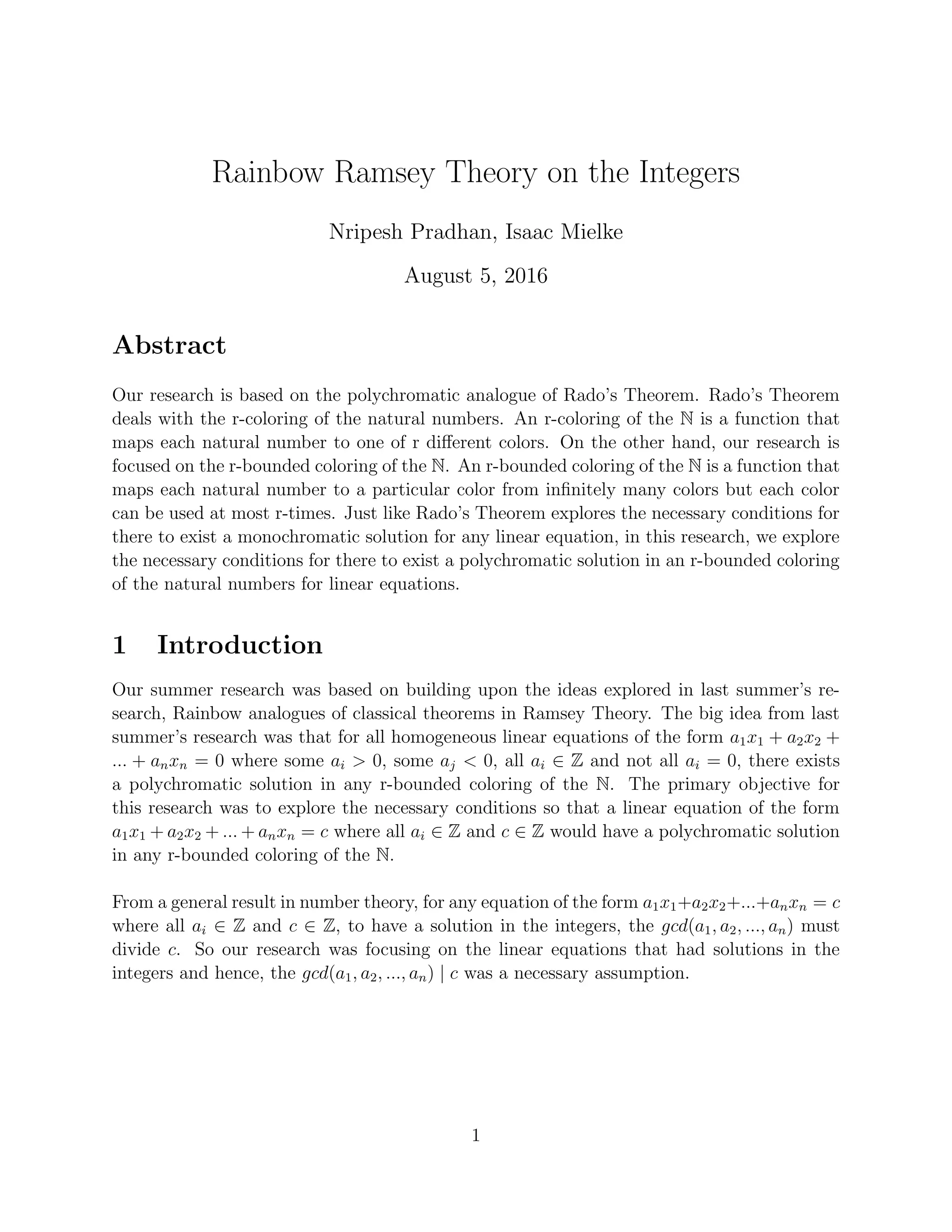
The document summarizes research on finding polychromatic solutions to linear equations in an r-bounded coloring of the natural numbers. The research builds on previous work exploring rainbow analogues of classical Ramsey theory results. Key findings include: 1) Theorems were proven showing that for equations of the form ax-by=c with integers a,b,c and gcd(a,b)|c, there exists a polychromatic solution in any r-bounded coloring. 2) Explicit recurrence relations and formulas were defined to generate chains of solutions to equations with two variables. 3) The results for two variables were used to show polychromatic solutions exist for equations with three variables of the form a1

1. Rainbow Ramsey Theory on the Integers
Nripesh Pradhan, Isaac Mielke
August 5, 2016
Abstract
Our research is based on the polychromatic analogue of Rado’s Theorem. Rado’s Theorem
deals with the r-coloring of the natural numbers. An r-coloring of the N is a function that
maps each natural number to one of r different colors. On the other hand, our research is
focused on the r-bounded coloring of the N. An r-bounded coloring of the N is a function that
maps each natural number to a particular color from infinitely many colors but each color
can be used at most r-times. Just like Rado’s Theorem explores the necessary conditions for
there to exist a monochromatic solution for any linear equation, in this research, we explore
the necessary conditions for there to exist a polychromatic solution in an r-bounded coloring
of the natural numbers for linear equations.
1 Introduction
Our summer research was based on building upon the ideas explored in last summer’s re-
search, Rainbow analogues of classical theorems in Ramsey Theory. The big idea from last
summer’s research was that for all homogeneous linear equations of the form a1x1 + a2x2 +
... + anxn = 0 where some ai > 0, some aj < 0, all ai ∈ Z and not all ai = 0, there exists
a polychromatic solution in any r-bounded coloring of the N. The primary objective for
this research was to explore the necessary conditions so that a linear equation of the form
a1x1 + a2x2 + ... + anxn = c where all ai ∈ Z and c ∈ Z would have a polychromatic solution
in any r-bounded coloring of the N.
From a general result in number theory, for any equation of the form a1x1+a2x2+...+anxn = c
where all ai ∈ Z and c ∈ Z, to have a solution in the integers, the gcd(a1, a2, ..., an) must
divide c. So our research was focusing on the linear equations that had solutions in the
integers and hence, the gcd(a1, a2, ..., an) | c was a necessary assumption.
1

2. 2 Two Variables
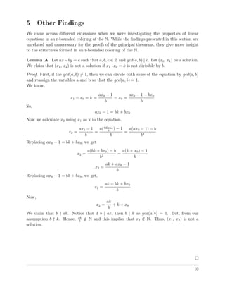
After looking at and finding solutions for equations of the form ax − by = c where a, b, c ∈ Z
and gcd(a, b) | c, we were fairly confident that all equations of that form would have a
polychromatic solution in any r-bounded coloring of the N. The idea behind finding polychro-
matic solution was first finding a set of ordered pair of solution of the form {(k1, k2), (k2, k3), ...(kr, kr+1).}
where ki = kj if and only if i = j. After we find such a set of ordered pair of solution, we
begin to color each ki sequentially. At any point, if ki and ki+1 have different colors, (ki, ki+1)
will be a polychromatic solution. From the Pigeonhole principle, each color can be used at
most r times and there are r + 1 kis to color. Thus, there exists an ordered pair (ki, ki+1)
such that ki and ki+1 have different colors and hence, we will have found a polychromatic
solution for our given equation ax − by = c.
The challenge was, however, to find a chain k1, k2, ...kr, kr+1 where for each i ∈ [r], (ki, ki+1)
is a solution. For most equations, we found such chains of length 4 or more but, it was
very difficult to find chains of length say, 100. Instead of manually writing out solutions and
looking for chains, we defined a recurrence relation from the equation and formally stated
and proved two conjectures that would simplify the process of finding such chains.
Theorem 0. Given any equation of the form ax − by = c where a, b, c ∈ Z and gcd(a, b) | c,
and a chain k1, k2, ...kr, kr+1 where for each i ∈ [r], (ki, ki+1) is a solution, there exists a
polychromatic solution for the equation ax − by = c for any r-bounded coloring of the N.
Proof. Given the chain k1, k2, ...kr, kr+1 , we begin to color each ki sequentially. At any
point, if ki and ki+1 have different colors, (ki, ki+1) will be a polychromatic solution. From
the Pigeonhole principle, each color can be used at most r times and there are r + 1 kis to
color. Thus, there exists an ordered pair (ki, ki+1) such that ki and ki+1 have different colors
and hence, we will have found a polychromatic solution for our given equation ax − by = c.
Definition 1. Given any equation of the form ax−by = c where a, b, c ∈ Z and gcd(a, b) | c,
we define T : Q → Q by T(x) = ax−c
b
.
Observation 0. We want our chain of solutions to be unique.That means, given a chain
k1, k2, ...kr, kr+1, for all 0 ≤ i ≤ r, we have ki = ki+1. However, if a = b and c = 0, then the
chain of solutions is not unique.
Notice that,
T(x) =
ax − c
b
=
ax
a
= x.
Since the function fixes x for all x ∈ N, in order to generate unique solutions, either a = b
or c = 0.
Notation: Let x = x0 and T(i)
(x) = xi+1 for all i ∈ N.
2

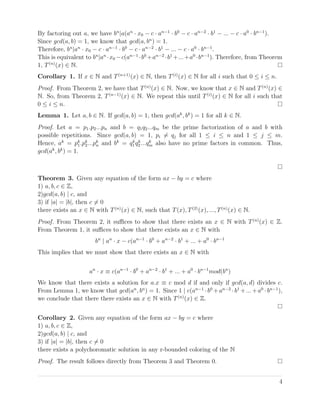
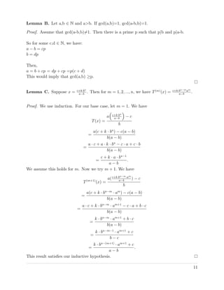
3. Theorem 1. Given any equation of the form ax − by = c where a, b, c ∈ Z and gcd(a, b) | c,
we define T : Q → Q by T(x) = ax−c
b
. Then, for any x0 ∈ N, we have
T(n)
(x0) =
an
· x0 − c(an−1
· b0
+ an−2
· b1
+ ... + a0
· bn−1
)
bn
.
Proof. First, if the gcd(a, b) = 1, then we can divide both sides of the equation by gcd(a, b)
and reassign the variables a and b so that the gcd(a, b) = 1.
We use induction.
For our base case, let n = 1. We have the following:
x1 =
a · x0 − c(a0
· b0
)
b1
=
a · x0 − c
b
.
Assume this holds for xn. We know that for any arbitrary (x, y) solution, y = ax−c
b
. If we
let y = xn+1, we have xn+1 = axn−c
b
. We can rewrite this as
xn+1 =
a[ 1
bn (an
· x0 − c(an−1
· b0
+ an−2
· b1
+ ... + a0
· bn−1
))] − c
b
=
an+1
· x0 − c(an
· b0
+ an−1
· b1
+ ... + a1
· bn−1
) − c
bn+1
=
an+1
· x0 − c(an
· b0
+ an−1
· b1
+ ... + a0
· bn
)
bn+1
.
This result satisfies our inductive hypothesis. Therefore,
xn =
an
· x0 − c(an−1
· b0
+ an−2
· b1
+ ... + a0
· bn−1
)
bn
.
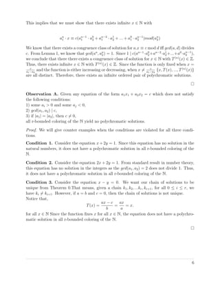
Theorem 2. If x0 ∈ N and T(n+1)
(x0) ∈ N, then T(n)
(x0) ∈ N.
Proof. First, if the gcd(a, b) = 1, then we can divide both sides of the equation by gcd(a, b)
and reassign the variables a and b so that the gcd(a, b) = 1.
Suppose x0 ∈ N and T(n+1)
(x0) ∈ N. Then, we will show that T(n)
(x0) ∈ N.
We know from Theorem 1 that,
T(n+1)
(x0) ∈ N =
an+1
· x0 − c(an
· b0
+ an−1
· b1
+ ... + a0
· bn
)
bn+1
.
Therefore, bn+1
|an+1
· x0 − c(an
· b0
+ an−1
· b1
+ ... + a0
· bn
).
This implies that bn
|an+1
· x0 − c(an
· b0
+ an−1
· b1
+ ... + a0
· bn
).
By expanding, we have bn
|an+1
· x0 − c · an
· b0
− c · an−1
· b1
− ... − c · a0
· bn
.
We know that bn
|c · bn
, so bn
|an+1
· x0 − c · an
· b0
− c · an−1
· b1
− ... − c · a1
· bn−1
.
3

4. By factoring out a, we have bn
|a(an
· x0 − c · an−1
· b0
− c · an−2
· b1
− ... − c · a0
· bn−1
).
Since gcd(a, b) = 1, we know that gcd(a, bn
) = 1.
Therefore, bn
|an
· x0 − c · an−1
· b0
− c · an−2
· b1
− ... − c · a0
· bn−1
.
This is equivalent to bn
|an
·x0 −c(an−1
·b0
+an−2
·b1
+...+a0
·bn−1
). Therefore, from Theorem
1, T(n)
(x) ∈ N.
Corollary 1. If x ∈ N and T(n+1)
(x) ∈ N, then T(i)
(x) ∈ N for all i such that 0 ≤ i ≤ n.
Proof. From Theorem 2, we have that T(n)
(x) ∈ N. Now, we know that x ∈ N and T(n)
(x) ∈
N. So, from Theorem 2, T(n−1)
(x) ∈ N. We repeat this until T(i)
(x) ∈ N for all i such that
0 ≤ i ≤ n.
Lemma 1. Let a, b ∈ N. If gcd(a, b) = 1, then gcd(ak
, bk
) = 1 for all k ∈ N.
Proof. Let a = p1.p2...pn and b = q1q2...qm be the prime factorization of a and b with
possible repetitions. Since gcd(a, b) = 1, pi = qj for all 1 ≤ i ≤ n and 1 ≤ j ≤ m.
Hence, ak
= pk
1.pk
2...pk
n and bk
= qk
1 qk
2 ...qk
m also have no prime factors in common. Thus,
gcd(ak
, bk
) = 1.
Theorem 3. Given any equation of the form ax − by = c where
1) a, b, c ∈ Z,
2)gcd(a, b) | c, and
3) if |a| = |b|, then c = 0
there exists an x ∈ N with T(n)
(x) ∈ N, such that T(x), T(2)
(x), ..., T(n)
(x) ∈ N.
Proof. From Theorem 2, it suffices to show that there exists an x ∈ N with T(n)
(x) ∈ Z.
From Theorem 1, it suffices to show that there exists an x ∈ N with
bn
| an
· x − c(an−1
· b0
+ an−2
· b1
+ ... + a0
· bn−1
This implies that we must show that there exists an x ∈ N with
an
· x ≡ c(an−1
· b0
+ an−2
· b1
+ ... + a0
· bn−1
mod(bn
)
We know that there exists a solution for a.x ≡ c mod d if and only if gcd(a, d) divides c.
From Lemma 1, we know that gcd(an
, bn
) = 1. Since 1 | c(an−1
·b0
+an−2
·b1
+...+a0
·bn−1
),
we conclude that there there exists an x ∈ N with T(n)
(x) ∈ Z.
Corollary 2. Given any equation of the form ax − by = c where
1) a, b, c ∈ Z,
2)gcd(a, b) | c, and
3) if |a| = |b|, then c = 0
there exists a polychoromatic solution in any r-bounded coloring of the N
Proof. The result follows directly from Theorem 3 and Theorem 0.
4

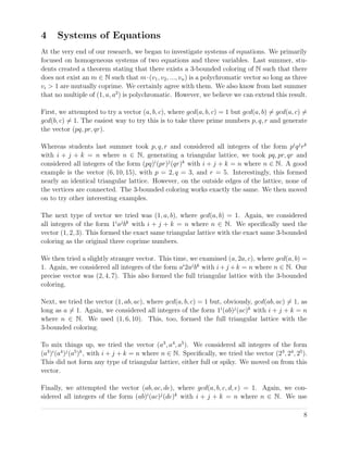
5. 3 Three variables
After proving the result in two variables, we moved on to linear equations with three variables.
Using the result from two variables, we show that for all linear equation of the form a1x1 +
a2x2 + a3x3 = c with all ai ∈ Z − [0] and gcd(a1, a2, a3) | c with some ai > 0, some ai < 0,
there exists a polychromatic solution in any r-bounded coloring of the N.
Lemma 2. Given any equation of the form a1x1 + a2x2 = c where a1, a2, c ∈ Z and
gcd(a1, a2) | c, we define T : Q → Q by T(x) = a1x1−c
−a2
. This function T : Q → Q is
an injective function.
Proof. Let T(k1) = T(k2) for arbitrary k1, k2 ∈ Q. Then,
a1k1 − c
−a2
=
a1k2 − c
−a2
Since a2 = 0, we have
a1k1 − c = a1k2 − ca1k1 = a1k2
Since a1 = 0, we have k1 = k2. Hence, T is injective.
Theorem A. Given any equation of the form a1x1 + a2x2 = c which satisfies the following
conditions:
1) some ai > 0 and some aj < 0,
2) gcd(a1, a2) | c,
3) if |a1| = |a2|, then c = 0
there exists an infinite ordered pair of polychromatic solutions in an r-bounded coloring of
the natural numbers.
Proof. First, if the gcd(a1, a2) = 1, then we can divide both sides of the equation by
gcd(a1, a2) and reassign the variables a and b so that the gcd(a1, a2) = 1.
We break down the proof into two cases.
Case 1. When |a1| = |a2|
From condition 3, we have that c = 0. Without loss of generality, we can assume a1 > 0
and a2 < 0. Thus, (2c, c), (3c, 2c), (4c, 3c), ...) are all solution in the natural numbers. Since
c = 0, we have that for all k ∈ N, (k + 1)c = kc. Thus, the chain of solutions c, 2c, 3c, 4c, ...
are all distinct. Since {(k + 1)c, kc} is a solution for all k ∈ N, there exists an infinite set of
polychromatic solutions.
Case 2. When |a1| = |a2|
When x = T(x), we have a1x − a2x = c. Thus, when x = c
a1−a2
, x = T(x). Since |a1| = |a2|,
only x = c
a1−a2
is fixed by the recurrence function.
From Theorem 2, it suffices to show that there exists infinite x ∈ N with T(n)
(x) ∈ Z. From
Theorem 1, it suffices to show that there exists infinite x ∈ N with
an
2 | an
1 · x − c(an−1
1 · a0
2 + an−2
1 · a1
2 + ... + a0
1 · an−1
2 )
5

6. This implies that we must show that there exists infinite x ∈ N with
an
1 · x ≡ c(an−1
1 · a0
2 + an−2
1 · a1
2 + ... + a0
1 · an−1
2 )mod(an
2 )
We know that there exists a congruence class of solution for a.x ≡ c mod d iff gcd(a, d) divides
c. From Lemma 1, we know that gcd(an
, an
2 ) = 1. Since 1 | c(an−1
·a0
2+an−2
·a1
2+...+a0
·an−1
2 ),
we conclude that there there exists a congruence class of solution for x ∈ N with T(n)
(x) ∈ Z.
Thus, there exists infinite x ∈ N with T(n)
(x) ∈ Z. Since the function is only fixed when x =
c
a1−a2
and the function is either increasing or decreasing, when x = c
a1−a2
{x, T(x), ..., T(n)
(x)}
are all distinct. Therefore, there exists an infinite ordered pair of polychromatic solutions.
Observation A. Given any equation of the form a1x1 + a2x2 = c which does not satisfy
the following conditions:
1) some ai > 0 and some aj < 0,
2) gcd(a1, a2) | c,
3) if |a1| = |a2|, then c = 0,
all r-bounded coloring of the N yield no polychromatic solutions.
Proof. We will give counter examples when the conditions are violated for all three condi-
tions.
Condition 1. Consider the equation x + 2y = 1. Since this equation has no solution in the
natural numbers, it does not have a polychromatic solution in all r-bounded coloring of the
N.
Condition 2. Consider the equation 2x + 2y = 1. From standard result in number theory,
this equation has no solution in the integers as the gcd(a1, a2) = 2 does not divide 1. Thus,
it does not have a polychromatic solution in all r-bounded coloring of the N.
Condition 3. Consider the equation x − y = 0. We want our chain of solutions to be
unique from Theorem 0.That means, given a chain k1, k2, ...kr, kr+1, for all 0 ≤ i ≤ r, we
have ki = ki+1. However, if a = b and c = 0, then the chain of solutions is not unique.
Notice that,
T(x) =
ax − c
b
=
ax
a
= x.
for all x ∈ N Since the function fixes x for all x ∈ N, the equation does not have a polychro-
matic solution in all r-bounded coloring of the N.
6

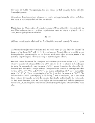
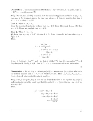
7. Theorem B. Given any r-bounded coloring of the N and any equation of the form a1x1 +
a2x2 + a3x3 = c with all ai ∈ Z − [0] and gcd(a1, a2, a3) | c with some ai > 0, some ai < 0,
we can find a polychromatic solution in any r-bounded coloring of the N.
Proof. First, if the gcd(a1, a2, a3) = 1, then we can divide both sides of the equation by
gcd(a1, a2, a3) and renumber the a s so that gcd(a1, a2, a3) = 1.
Since we have three ai with with some ai > 0, some ai < 0, we can renumber the a s and
rearrange the equation to get, a1x1 + a2x2 = c − a3x3 such that a1 > 0 and a2 < 0.
Notice that there exists a congruence class of x3, such that c ≡ a3x3 mod gcd(a1, a2) as
gcd(a3, gcd(a1, a2)) = gcd(a1, a2, a3) = 1. Pick a value for x3 such that c − a3x3 = 0. Now,
x3 has a particular color. From Theorem A, we know that a1x1 + a2x2 = c − a3x3 has an
infinite set of ordered pair of polychromatic solutions. From Lemma 2 and the property of
a function, we know that each k ∈ N can appear at most two times in the infinite set of
ordered pair of polychromatic solutions. So, from the Pigeonhole principle, we can pick x1
and x2 such that they both have different colors than that of x3 as the color of x3 can appear
at most r times. Thus, we can ensure that x1, x2, x3 all have different colors.
7

8. 4 Systems of Equations
At the very end of our research, we began to investigate systems of equations. We primarily
focused on homogeneous systems of two equations and three variables. Last summer, stu-
dents created a theorem stating that there exists a 3-bounded coloring of N such that there
does not exist an m ∈ N such that m·(v1, v2, ..., vn) is a polychromatic vector so long as three
vi > 1 are mutually coprime. We certainly agree with them. We also know from last summer
that no multiple of (1, a, a2
) is polychromatic. However, we believe we can extend this result.
First, we attempted to try a vector (a, b, c), where gcd(a, b, c) = 1 but gcd(a, b) = gcd(a, c) =
gcd(b, c) = 1. The easiest way to try this is to take three prime numbers p, q, r and generate
the vector (pq, pr, qr).
Whereas students last summer took p, q, r and considered all integers of the form pi
qj
rk
with i + j + k = n where n ∈ N, generating a triangular lattice, we took pq, pr, qr and
considered all integers of the form (pq)i
(pr)j
(qr)k
with i + j + k = n where n ∈ N. A good
example is the vector (6, 10, 15), with p = 2, q = 3, and r = 5. Interestingly, this formed
nearly an identical triangular lattice. However, on the outside edges of the lattice, none of
the vertices are connected. The 3-bounded coloring works exactly the same. We then moved
on to try other interesting examples.
The next type of vector we tried was (1, a, b), where gcd(a, b) = 1. Again, we considered
all integers of the form 1i
aj
bk
with i + j + k = n where n ∈ N. We specifically used the
vector (1, 2, 3). This formed the exact same triangular lattice with the exact same 3-bounded
coloring as the original three coprime numbers.
We then tried a slightly stranger vector. This time, we examined (a, 2a, c), where gcd(a, b) =
1. Again, we considered all integers of the form ai
2aj
bk
with i+j +k = n where n ∈ N. Our
precise vector was (2, 4, 7). This also formed the full triangular lattice with the 3-bounded
coloring.
Next, we tried the vector (1, ab, ac), where gcd(a, b, c) = 1 but, obviously, gcd(ab, ac) = 1, as
long as a = 1. Again, we considered all integers of the form 1i
(ab)j
(ac)k
with i + j + k = n
where n ∈ N. We used (1, 6, 10). This, too, formed the full triangular lattice with the
3-bounded coloring.
To mix things up, we tried the vector (a3
, a4
, a5
). We considered all integers of the form
(a3
)i
(a4
)j
(a5
)k
, with i + j + k = n where n ∈ N. Specifically, we tried the vector (23
, 24
, 25
).
This did not form any type of triangular lattice, either full or spiky. We moved on from this
vector.
Finally, we attempted the vector (ab, ac, de), where gcd(a, b, c, d, e) = 1. Again, we con-
sidered all integers of the form (ab)i
(ac)j
(de)k
with i + j + k = n where n ∈ N. We use
8

9. the vector (6, 10, 77). Unsurprisingly, this also formed the full triangular lattice with the
3-bounded coloring.
Although we do not understand why pq, pr, qr creates a strange triangular lattice, we believe
that there is more to the theorem from last summer.
Conjecture A. There exists a 3-bounded coloring of N such that there does not exist an
m ∈ N such that m · (v1, v2, ..., vn) is a polychromatic vector so long as v1 = v2 = ... = vn.
Thus, the integer system of equations
Ax = 0
yields no polychromatic solutions if ker A = Span(v) where each entry of v is unique.
Another interesting feature we found is that for some vector (a, b, c), where we consider all
integers of the form ai
bj
ck
with i + j + k = n where n ∈ N, each different n for this vector
fits together in a giant triangular lattice. In other words, each n just isolates a portion of an
infinitely large triangular lattice consisting of finite triangular lattices.
One last curious feature of the triangular lattice is that given some vector (a, b, c), again
where we consider all integers of the form ai
bj
ck
with i + j + k = n where n ∈ N, as long as
we know the values of a, b, c and the value of ai
bj
ck
, we can determine the values of i, j, k.
We know that each finite triangle within a triangular lattice consists of a triangle with the
vertices ai
bj
ck
, ai−1
bj+1
ck
, and ai−1
bj
ck+1
. By merely multiplying ai
bj
ck
by b
a
, we find the
value of ai−1
bj+1
ck
. Then, by multiplying ai
bj
ck
by c
a
, we find the value of ai−1
bj
ck+1
. We
can also find ai−1
bj+1
ck
by multiplying ai−1
bj
ck+1
by b
c
. This is because i+j +k = n for all of
these vertices. We can also move in the opposite direction by multiplying by the reciprocals.
As long as we have one value, we can complete its finite triangle and find the appropriate
values for i, j, k, allowing us to complete an arbitrarily large triangular lattice with this value
of n.
9

10. 5 Other Findings
We came across different extensions when we were investigating the properties of linear
equations in an r-bounded coloring of the N. While the findings presented in this section are
unrelated and unnecessary for the proofs of the principal theorems, they give more insight
to the structures formed in an r-bounded coloring of the N.
Lemma A. Let ax−by = c such that a, b, c ∈ Z and gcd(a, b) | c. Let (x0, x1) be a solution.
We claim that (x1, x2) is not a solution if x1 -x0 = k is not divisible by b.
Proof. First, if the gcd(a, b) = 1, then we can divide both sides of the equation by gcd(a, b)
and reassign the variables a and b so that the gcd(a, b) = 1.
We know,
x1 − x0 = k =
ax0 − 1
b
− x0 =
ax0 − 1 − bx0
b
So,
ax0 − 1 = bk + bx0
Now we calculate x2 using x1 as x in the equation.
x2 =
ax1 − 1
b
=
a(ax0−1
b
) − 1
b
=
a(ax0 − 1) − b
b2
Replacing ax0 − 1 = bk + bx0, we get
x2 =
a(bk + bx0) − b
b2
=
a(k + x0) − 1
b
x2 =
ak + ax0 − 1
b
Replacing ax0 − 1 = bk + bx0, we get,
x2 =
ak + bk + bx0
b
Now,
x2 =
ak
b
+ k + x0
We claim that b ak. Notice that if b | ak, then b | k as gcd(a, b) = 1. But, from our
assumption b k. Hence, ak
b
/∈ N and this implies that x2 /∈ N. Thus, (x1, x2) is not a
solution.
10

11. Lemma B. Let a,b ∈ N and a>b. If gcd(a,b)=1, gcd(a-b,b)=1.
Proof. Assume that gcd(a-b,b)=1. Then there is a prime p such that p|b and p|a-b.
So for some c,d ∈ N, we have:
a − b = cp
b = dp
Then,
a = b + cp = dp + cp =p(c + d)
This would imply that gcd(a,b) ≥p.
Lemma C. Suppose x = c+k·bn
a−b
. Then for m = 1, 2, ..., n, we have T(m)
(x) = c+k·bn−mam
a−b
.
Proof. We use induction. For our base case, let m = 1. We have
T(x) =
a c+k·bn
a−b
− c
b
=
a(c + k · bn
) − c(a − b)
b(a − b)
=
a · c + a · k · bn
− c · a + c · b
b(a − b)
=
c + k · a · bn−1
a − b
.
We assume this holds for m. Now we try m + 1. We have
T(m+1)
(x) =
a(c+k·bn−m·am
a−b
) − c
b
=
a(c + k · bn−m
· am
) − c(a − b)
b(a − b)
=
a · c + k · bn−m
· am+1
− c · a + b · c
b(a − b)
=
k · bn−m
· am+1
+ b · c
b(a − b)
=
k · bn−m−1
· am+1
+ c
b − c
=
k · bn−(m+1)
· am+1
+ c
a − b
.
This result satisfies our inductive hypothesis.
11

12. Observation 1. Given any equation of the form ax−by = c where a, b, c ∈ Z and gcd(a, b) |
c, if bn
x1 − x0, then xn+1 /∈ N.
Proof. We will do a proof by induction. Let the inductive hypothesis be that if bn
x1 − x0,
then xn+1 /∈ N. Lemma A proves the base case when n = 1 Now, we want to show that if
bn+1
x1 − x0, then xn+2 /∈ N.
Case 1. When bn
x1 − x0
From the inductive hypothesis, we know that xn+1 /∈ N. From Theorem 2 if xn+2 ∈ N, then
xn+1 ∈ N. Hence, we conclude that xn+2 /∈ N.
Case 2. When bn
| x1 − x0
We know that x1 − x0 = k · bn
for some k ∈ N. From Lemma B, we know that xn+1 =
k.an+c
a−b
∈ N.
Then,
xn+2 =
k·an+1+ac
a−b
− c
b
=
k · an+1
+ ac − ac + bc
b(a − b)
=
k · an+1
+ bc
b(a − b)
If xn+2 ∈ N, then b | (k.an+1
) as b | bc. But, if b | (k.an+1
), then b | k as gcd(b, an+1
) = 1
from Lemma B. Finally, if b | k , then bn+1
| x1 − x0, which contradicts our assumption.
Observation 2. Let ax − by = c where gcd(a, b) | c .Assume that (x0, x1) is a solution in
the natural numbers and x1 − x0 = k.br
where k,r ∈ N.. Then (x0,x1),(x1, x2),(x2,x3),...
(xr,xr+1) are all solutions in the natural numbers.
Proof. First, if the gcd(a, b) = 1, then we can divide both sides of the equation by gcd(a, b)
and reassign the variables a and b so that the gcd(a, b) = 1. Notice that x1 − x0 = k.br
so,
x0 = x1 − k.br
Then,
ax1 − k.a.br
− bx1 = 1
ax1 − bx1 = 1 + k.abr
x1(a − b) = 1 + k.abr
x1 =
1 + k.abr
a − b
12

13. Now we expect (x1, x2) to be a solution. For that, x2 ∈ N. We calculate x2 from the equation
to get,
ax1 − bx2 = 1
a(1 + k.abr
)
a − b
− bx2 = 1
bx2 =
a + k.a2
br
− a + b
ab
bx2 =
b + k.a2
.br
a − b
x2 =
1 + k.a2
.br−1
a − b
Notice that,
k.abr
≡ −1 mod(a-b)
a ≡ b mod(a-b)
So, k.a2
.br
≡ −b mod(a-b) From Lemma B, gcd(a − b, b) = 1. Hence, k.a2
.br−1
≡ −1 mod
(a-b) So, we conclude that x2 ∈ N
Similarly, x3 = 1+k.a3.br−2
a−b
∈ N xr+1 = 1+k.ar
a−b
∈ N.
Conjecture 1. Given any r-bounded coloring of the natural numbers and any equation of
the form a1x1 + a2x2 + ... + anxn = c with all ai ∈ Z − [0] and gcd(a1, a2, ..., an)|c with some
ai > 0 and some ai < 0, we can find a polychromatic solution in the natural numbers.
Conjecture 2. Given any equation of the form ax−by = c where a, b, c ∈ Z and gcd(a, b) | c,
for all x ∈ N, if T(x) = x, then there exists an n ∈ N with T(n)
(x) ∈ N.
6 Future Work
We have many ideas to extend this research within Rainbow Ramsey Theory. The most
obvious place to begin is by finishing our remaining conjectures. From there, the next
logical step is to expand our scope and examine all homogeneous linear systems, which we
believe will demonstrate similar properties as systems of equations with just two equations
and three variables. Ultimately, we would like to investigate non-homogeneous systems of
equations.
13

14. Acknowledgments
We would like to thank Professor Joseph Mileti, our faculty mentor, for his guidance and
patience. We would also like to thank Grinnell College for funding our project.
References
[1] Henry Ehrhard, David Kraemer, Boyd Monson, Yifei Zhang. Rainbow Ramsey Theory
on the Integers. Grinnell College, IA, 2015.
[2] Ronald L. Graham, Bruce L. Rothschild, Joel H. Spencer. Ramsey Theory. Wiley-
Interscience, 1990.
[3] Bruce M. Landman, Aaron Robertson. Ramsey Theory on the Integers. American Math-
ematical Society, RI, 2014.
14